Tsukasa Mizutani, Shunsuke Iwai (2024). Automated Method for Quantitative Measurement of Underground Construction Sites Using iPhone LiDAR Point Cloud Data. In: Human Factors in Design, Engineering, and Computing. AHFE Open Access, vol. 159, pp. 1760–1770. https://doi.org/10.54941/ahfe1005743
Electrical transmission methods vary globally between overhead and underground systems. Underground transmission is increasingly favored for several reasons, including landscape aesthetics, enhanced pedestrian safety, and disaster prevention. Overhead systems, while initially cheaper and easier to repair, pose substantial risks during disasters such as earthquakes, where utility poles may collapse, obstructing emergency response and increasing the likelihood of power outages. In contrast, underground systems mitigate these risks effectively.In regions with advanced pole-free electrification like Europe, utility infrastructure development predominantly favors underground installations to ensure both aesthetic and functional equality between gas and electrical systems. This approach has resulted in nearly complete underground utility coverage in major Western cities, contrasting sharply with Japan, where the transition from overhead to underground has been sluggish. This lag is due to post-WWII reconstruction policies which prioritized quick and stable overhead installations. Despite ongoing efforts, Japan's adoption of underground systems remains notably low.Globally, the construction of utility tunnels is promoted to optimize the use of underground space, particularly in urban centers where space is at a premium. These tunnels, housing essential services like electricity, water, and gas, are seen as a solution to urban underground congestion, a problem often referred to as the "Spaghetti problem." However, high costs and recent fiscal constraints have slowed the implementation of these systems in places like Japan.This research focuses on enhancing the construction efficiency of utility tunnels to expedite their adoption. This involves night-time construction operations including excavation, installation of conduits and "CC-Box" manholes, and subsequent backfilling. Such processes are labor-intensive and require pauses for measurement and documentation, making efficiency improvements critical.Our study leverages Light Detection and Ranging (LiDAR) technology to address these efficiency challenges. LiDAR point cloud data, employed in construction since 2004, has seen increased application following Apple's integration of LiDAR scanners in its 2020 iPad Pro and iPhone 12 Pro models. We aim to develop an algorithm to extract excavation sections from this data for precise volume measurements without reliance on Building Information Modeling (BIM).Our proposed method details techniques for measuring excavation dimensions (horizontal, vertical, and depth) at construction sites and discusses results from applying this method in field tests. These results indicate significant potential for enhancing measurement accuracy and reducing both labor costs and processing time. This research contributes to the field by providing a novel approach to utility tunnel excavation that utilizes advanced LiDAR technology for more efficient construction management and hazard prevention. The final sections of the paper summarize these findings and discuss their implications for future construction practices.
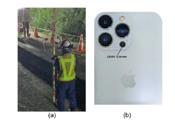
Underground transmission, which replaces utility poles with underground conduits, is increasingly preferred due to its aesthetic benefits, enhanced pedestrian safety, and reduced disaster risk (MLIT). Globally, utility tunnels are being constructed to efficiently use underground space for utilities such as electricity, water, and gas (Yang et al., 2016) (Wang et al., 2018). In Japan, transitioning to pole-free environments depends on developing these tunnels. However, their high cost and fiscal constraints have slowed progress. This research aims to improve utility tunnel construction efficiency, reducing costs and construction times. In Japan, tunnel construction involves nighttime stages of excavation, conduit installation, and backfilling, with frequent stops for measurements and documentation, necessitating improvements in efficiency (see Figure 1 (a)).
To address these challenges, we explore LiDAR technology (National Ocean Service), already used in construction for 3D modeling and quality
Automated Method for Quantitative Measurement 1761
inspection. Following Apple’s integration of LiDAR in iPad Pro and iPhone 12 Pro (see Figure 1 (b)), research has expanded, but the use of smartphone LiDAR for tunnel wall analysis is limited (Torkan et al., 2023). We previously proposed a segmentation method utilizing color information (Mizutani et al., 2024). By incorporating a wider range of analyses into this algorithm, we can enhance its robustness. We collected point cloud data at utility tunnel sites using an iPad Pro, aiming to develop an algorithm for accurately measuring excavation sections.
Figure 1: Measurement equipment – (a) example of conventional equipment in use (e.g., rulers, tapes, cameras, etc.), (b) iPhone device with a LiDAR camera.
Excavation Measurement Method The proposed method is fully automated and based on computational processes utilizing image processing, 3D point-cloud processing, signal processing and optimization techniques. The proposed method is applied to 3D data of excavations obtained using LiDAR (Light Detection and Ranging) scanners. Measurement of an excavation is generally done when the excavation is blank (1) or when objects (e.g., underground pipes) are embedded inside the excavation (2). Therefore, the proposed method is divided into two major phases – (1) measurement of blank excavation (Phase 1) and (2) measurement of excavation embedded with pipes (Phase 2). In this paper, we refer to excavations embedded with pipes as “excavations with pipes”. In Phase 1, measurement is executed on LiDAR data collected from a completely dug and void excavation, and the results are saved as future references for use in Phase 2. In Phase 2, measurement is executed on LiDAR data collected after construction objects (e.g., underground pipes) are placed inside the void excavation of Phase 1.
LiDAR data, represented as 3D points sampled and equally spaced along the X and Y axes, may not contain values for every grid point and can have multiple points with the same X and Y coordinates. In construction
1762 Mizutani and Iwai
site excavations, a rotation is generally observed between the LiDAR data X-Y plane and the excavation transversal-longitudinal plane, and the main excavation may connect to unmeasured side excavations.
Phase 1: Measurement of Blank Excavation In Phase 1, the proposed method executes a series of processes on LiDAR data to calculate the outputs. In addition, it saves specific results to use as a reference while calculating outputs for the same excavation after it is turned into an excavation with pipes. For processing LiDAR data in this phase, we divide the workflow into the following six steps.
Step 1: Segment Excavation Area We use MLESAC (Torr et al., 2000) for plane fitting to segment LiDAR points of the ground plane in the data. MLESAC estimates a plane with the most inliers within a threshold distance and labels points as inliers or outliers. For excavation data, ground plane points are labeled as inliers. Using the segmented ground plane, we empirically determine a threshold to separate points above and below it, labeling the points below as the excavation area.
Step 2: Remove the Side Excavations To address the presence of adjacent small excavations in the segmented LiDAR data, we employ a 3D point cloud processing technique to isolate the main excavation. This technique segments the excavation point cloud into clusters based on Euclidean distance. To remove adjacent areas and side excavations, we convert the LiDAR points into a binary image on the X-Y plane, where each pixel value is set to 1 if it corresponds to a LiDAR point and 0 otherwise. This binary image, usually sparse, is used to identify the main excavation borders using image processing techniques and the Radon transform, ensuring only the main excavation area is considered during measurement.
Step 3: Rotate the Main Excavation In this step, we segment the points on the bottom plane of the main excavation area using the MLESAC method. Outliers are removed based on a neighborhood distance metric. We then calculate the direction vector of the bottom plane to determine the rotation angle θ, aligning the transversal and longitudinal directions with the X and Y axes of the LiDAR data. This rotation is applied to the 3D points of the main excavation, ensuring accurate alignment for further analysis.
Step 4: Segment Each Wall and Bottom Plane from the Rotated Main Excavation To accurately segment the bottom plane and sidewalls of an excavation, we apply a line scanning technique along the Y-axis to extract transversal lines. By defining cavity areas with percentile-based thresholds, we detect walls by identifying the first yi value where the number of points exceeds a threshold. We then employ optimal change-point detection to fine-tune the left and right sidewall borders. Finally, we use straight-line fitting to refine these borders, ensuring the extracted points lie accurately on the bottom plane.
Automated Method for Quantitative Measurement 1763
Step 5: Get Reference Points on the Ground Plane In Step 5, we prepare to calculate the depth of the bottom plane from the ground plane by using scanned lines along the Y-axis. The ground plane is rotated according to the main excavation’s angle, and objects bridging the excavation sides are removed. For each scanned line, the nearest points on the ground to the left and right border points of the main excavation are detected. If no valid points are found, the nearest previously calculated reference point is used.
Step 6: Calculate the Metrics To calculate length and width, the bottom plane segmented in Step 3 is used. Length is determined by calculating the distance between border points on each longitudinal scanned line, while width is calculated similarly for transversal lines. Average depth is obtained by averaging the Z coordinate values of points on a scanned line and subtracting the Z coordinates of reference points on the ground plane. Depth mesh and length mesh are generated by aggregating Z coordinate values and distributing them on a 2D mesh based on X and Y coordinates. Data from Phase 1, including coordinates of the bottom plane and rotation angles, are saved as reference for Phase 2 measurements.
Phase 2: Measurement of Excavation with Pipes In this section, we describe Phase 2 of the proposed measurement method, where the object in question for measurement is excavation with pipes. In Phase 2, the proposed method utilizes the data saved during the procedures of Phase 1 and executes another series of image and 3D data processing on LiDAR data for calculating outputs regarding excavation with pipes.
Step 1: Use Reference Data to Extract the Bottom Plane In this step, we use the MLESAC-based plane fitting method to segment the main excavation area in the Phase 2 dataset. By leveraging the X and Y coordinate values from the Phase 1 Reference Data, we simplify the calculations in Phase 2 through a range-matching algorithm. This allows us to extract the bottom plane from the Phase 2 dataset. Subsequently, we estimate the rotation angle of the main excavation and apply this rotation to align the datasets from both phases. Finally, we perform outlier removal on the Phase 2 bottom plane.
Step 2: Measure Underground Pipes In this step, we measure the dimensions of underground pipes in an excavation using the Phase 2 dataset. We use image morphological methods to interpolate missing areas in the LiDAR data and apply a 2D median filter for smoothing. The smoothed and interpolated image, called the “Final Bottom Plane,” is used to calculate pipe metrics. We identify the endpoints of pipes by detecting sharp changes in the longitudinal scanned lines and compute the pipe end curves. The highest value of pipe lengths is determined by finding the maximum differences between the top and bottom endpoints.
1764 Mizutani and Iwai
Step 3: Get Reference Points on the Ground Plane Step 4: Calculate the Metrics The methods used in Step 3 and Step 4 are the same as those described in Phase1. In Step 3, we find out the reference points on ground plane using the same methods described in Step5 of Phase1. On the other hand, in Step 4, the output metrics, are calculated using the points on the Final Bottom Plane and sidewalls using the same methods in Step6 of Phase1.
The LiDAR dataset for excavations with pipes is referred to as the “Phase 2 dataset”, and the bottom plane from Phase 1 is the “Phase 1 bottom plane”.
RESULTS AND DISCUSSION
In this chapter, we present a set of results obtained by applying our proposed method on actual data from a construction site and discuss the possibility of drastic improvement in construction site measurement in terms of accuracy, labor cost, and processing time.
In the next sections, we describe figures displaying measurement results and provide remarks on the obtained results. These intermediate outputs basically consist of detected areas, such as the bottom plane, sidewalls, etc., which are necessary for calculating the final outputs.
For the convenience of display, we show two figures for each construction site measurement, showing the intermediate outputs and the final outputs separately. For the convenience of discussion, we call this set of two figures “Result Display”.
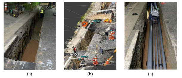
Figure 3 and Figure 4 are the Result Display of Phase 1 for the blank excavation shown in Figure 2 (a). Here, Figure 2 (a) is an example of an excavation. Figure 5 and Figure 6 show the Result Display of Phase 2 for the excavation with pipes.
Figure 2: Actual images of the construction site from where the LiDAR data used in this chapter were acquired – (a) blank excavation, (b) LiDAR data visualization of (a), (c) excavation with pipes.
In this paper, we do a visual assessment of our proposed method using graphical representations of detected areas in different colors. We assume that for any of the final outputs, if the area or segment of the excavation required for calculating those outputs is detected with satisfactory accuracy in visual assessment, then the accuracy of the calculated outputs will be the
Automated Method for Quantitative Measurement 1765
same as that of the LiDAR scanner. Figure 2 shows a set of actual images of excavations taken at construction sites, which were scanned to validate the efficiency of our proposed method.
Remarks on Intermediate Outputs In this section, we provide remarks on the visual assessment of the intermediate outputs obtained using our proposed method. Intermediate outputs are collected in Phase 1 and Phase 2.
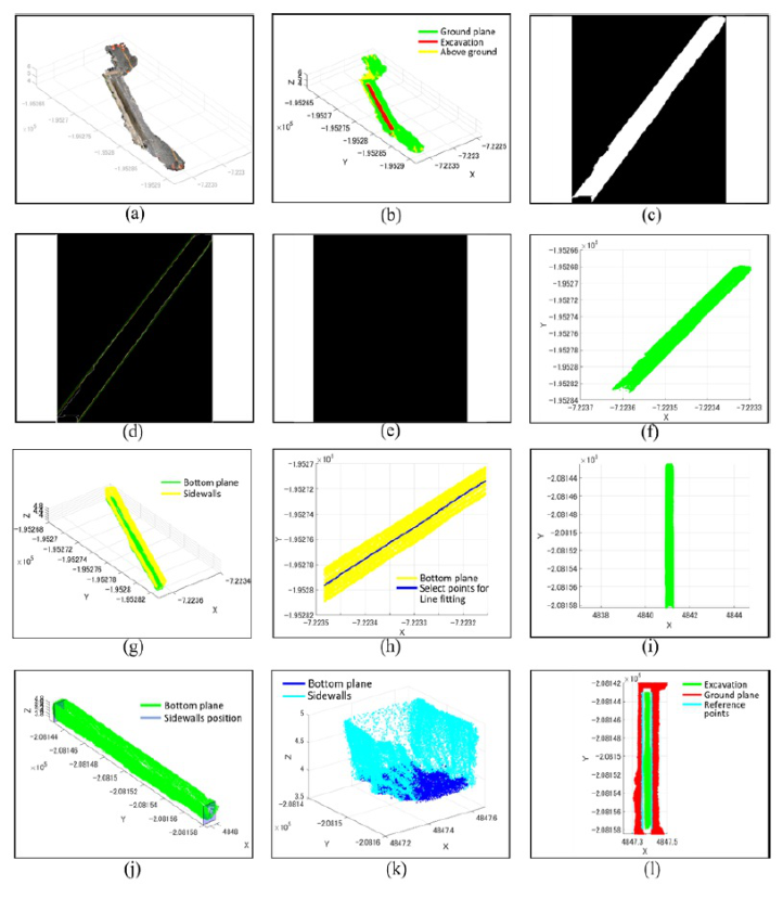
Figure 3 displays the intermediate outputs for an excavation of regular type, as shown in Figure 2 (a). The intermediate outputs consist of several visual displays segmented ground plane, excavation and objects above the plane, initially segmented bottom plane of an excavation, image processing results on detecting main excavation edges and side excavations, points acquired for calculating bottom plane rotation, rotated bottom plane, segmented sidewalls, segmented bottom plane, and detected reference points on the ground plane.
The results in Figure 3 (b) imply that the excavation segmentation technique based on 3D plane fitting (Step1 of Phase1) separates the excavation, ground plane and objects on the plane with considerable efficiency. In addition, Figure 3 (g) shows that the 3D plane fitting technique is useful in separating the bottom plane from the sidewalls of an excavation.
Figure 3 (h), (i) shows that for excavations, our approach in rotation angle estimation and data alignment to the X-axis and Y-axis of LiDAR coordinates performs with acceptable accuracy. We show that in addition to aligning the bottom plane, our approach collects points around the longitudinal middle line of a bottom plane accurately.
Figure 3 (j) shows that the two sidewalls on longitudinal ends are detected with considerable accuracy. Similarly, Figure 3 (k) shows that the bottom plane and transversal sidewalls are separated correctly. The points on these separated bottom planes are then used in length, width, depth and depth mesh calculation for outputs. On the other hand, the points on the separated sidewalls are used in calculating width mesh and length mesh for outputs. Figure 3 (l) shows that the reference points on ground plane are detected correctly.
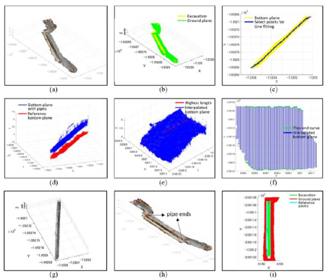
The intermediate outputs obtained in Phase 2 are displayed in Figure 5. Figure 5 (b) shows that the performance of the excavation segmentation technique based on 3D plane fitting in Phase 2 is comparable to that in Phase 1 in terms of excavation. A similar impression can be obtained regarding bottom plane rotation results in Phase 2 from Figure 5 (c) excavation. Figure 5 (d) shows that for excavations, the reference bottom plane saved during Phase 1 is well aligned to the obtained bottom plane in Phase 2 in terms of X and Y coordinates.
The pipe ends processing results shown in Figure 5 (e)-(h) for excavations, imply that the pipe topologies are detected quite accurately. Therefore, the dimensions of pipes calculated in this paper are estimated with acceptable accuracy. Finally, Figure 5 (i) shows that the reference points on ground plane are detected correctly.
1766 Mizutani and Iwai
Figure 3: Intermediate outputs of the measurement process of Phase 1 regarding a regular type of blank excavation – (a) LiDAR data view with actual colors, (b) LiDAR data view with segmented areas (green: ground plane, yellow: above ground, red: excavation), (c) LiDAR data juxtaposed on 2D image plane and morphological operations applied on it, (d) boundary lines of excavation estimated using edge detection, (e) segmented side excavation areas on image, (f) display of main excavation (green), side excavation (red) and their connecting lines (blue), (g) LiDAR data view of excavation area only with different colors for coarsely segmented areas (yellow: side walls, green: bottom plane), (h) X and Y coordinates of bottom plane (yellow) and points selected for straight line fitting (blue) to estimate rotation angle, (i) bottom plane after rotation, (j) side walls detected on the longitudinal direction, (k) bottom plane and side walls after fine tuning (Step4 in Phase 1), (l) reference points on ground plane.
Automated Method for Quantitative Measurement 1767
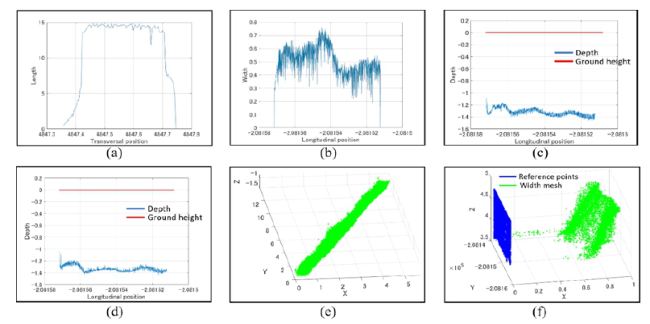
Figure 4: Measurement outputs of Phase 1 regarding a blank excavation – (a) length along the transversal direction, (b) width along longitudinal direction, (c) average depth along longitudinal direction regarding the reference points on left side, (d) average depth along longitudinal direction regarding the reference points on right side, (e) depth mesh, (f) width mesh regarding left side wall (blue: reference points on side walls, green: width value, i.e., distance of right side wall from each reference points).Figure 5: Intermediate outputs and some measurement outputs of Phase 2 regarding an excavation with pipes – (a) LiDAR data view with actual colors, (b) LiDAR data view with segmented areas (green: ground plane, yellow: above ground, red: excavation), (c) X and Y coordinates of bottom plane (yellow) and points selected for straight line fitting (blue) to estimate rotation angle, (d) bottom plane of excavation with pipes (blue) and reference bottom plane of blank excavation (red), (e) pipe area after image morphology (blue points) and the highest length of pipes (red straight line), (f) pipe ends along transversal direction (green curves), (g) LiDAR view of segmented pipes, (h) detected both ends of pipes shown in full view of LiDAR data, (i) reference points on ground plane.
1768 Mizutani and Iwai
Remarks on Final Outputs of the Proposed Method
Figure 4 summarizes the outputs obtained in Phase 1 for excavation. Figure 4 (a)-(d) shows examples of calculated length, width, and depth (regarding both the left and right edges) of the bottom planes of an excavation. On the other hand, Figure 4 (e)-(f) shows examples of depth mesh and width mesh for an excavation.
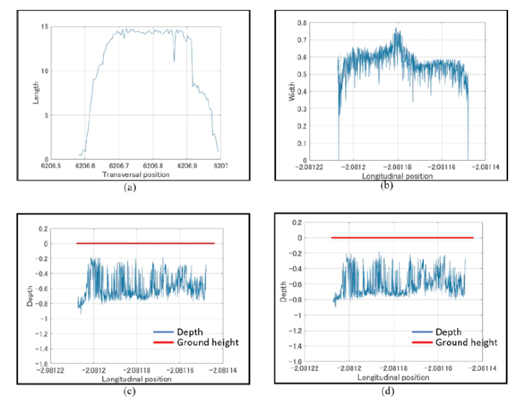
The accuracy of these metrics shown in Figure 4 (a)-(f) depends on how accurately the bottom plane and sidewalls of an excavation and reference points on the ground planes are detected during the operations for obtaining intermediate outputs. Therefore, we can say that these metrics are calculated with accuracy similar to that of the LiDAR scanner. Figure 6 summarizes the outputs obtained in Phase 2 for excavation. Figure 6 (a)-(d) shows examples of calculated length, width, and depth (regarding both the left and right edge) of the bottom planes.
Figure 6: Measurement outputs of Phase 2 regarding a regular type of excavation with pipes – (a) length along transversal direction, (b) width along longitudinal direction, (c) average depth along longitudinal direction regarding the reference points on left side, (d) average depth along longitudinal direction regarding the reference points on right side.
Automated Method for Quantitative Measurement 1769
Accuracy and Calculation Cost We conclude that because the intermediate outputs are detected with considerable accuracy in terms of visual assessment, the accuracy of the final outputs of our method is the same as that of the LiDAR scanner used in measurement. Because we used a consumer-grade scanner here, we also conclude that the accuracy of our proposed method is expected to increase proportionately when industry-grade LiDAR scanners with much higher accuracy are used.
The computational time we observed in Phase 1 and Phase 2 are summarized in Table 1. We found that the computational time depends on some specs of an excavation (e.g., type, dimensions, number of points available for width and length mesh, etc).
From Table 1, we can say that for a fifteen meters long excavation, our proposed automated measurement method can calculate necessary metrics with computational time on the order of 10 seconds after LiDAR scanning is complete. Compared to conventional manual measurements using rulers and tapes, which are customary practice in construction sites, this performance is a very big improvement.
Table 1. Computational cost.
Table available in the original PDF paper.
Dimension (m×m × m)
Number of Points in Width/ Length Mesh
Time-Phase 1 (Sec.)
Time-Phase 2 (Sec.)
0.8×15×1.5 19245 28.30 28.64
CONCLUSION
In this paper, we proposed a 3D data measurement method for calculating useful metrics of construction sites and presented a set of measurement results using examples of excavations and underground pipes. We showed that our proposed method can measure various metrics of an excavation with remarkably high accuracy and density. We also conclude that our method preserves the measurement accuracy of the LiDAR device used in scanning, and thus ensures higher accuracy when a higher-graded scanner is employed in measurement.
We expect that this method will bring a revolutionary change in the field of construction management. Because all the major drawbacks of conventional manual measurements, e.g., low accuracy, nominal measurement spots, long processing time, and tedious labor, can be drastically improved using our proposed method.
Future studies may include further detailed measurement, e.g., detecting individual objects inside an excavation, measuring individual pipes, etc.
ACKNOWLEDGMENT
This work was supported by Council for Science, Technology and Innovation (CSTI), Cross-ministerial Strategic Innovation Promotion Program (SIP), the
1770 Mizutani and Iwai
3rd period of SIP "Smart Infrastructure Management System" Grant Number JPJ012187 (Funding agency: Public Works Research Institute), and the Grant JPMJFR215R in JST (Japan Science and Technology Agency) FOREST (Fusion Oriented REsearch for disruptive Science and Technology) Program (Grant Recipient: Tsukasa MIZUTANI).
REFERENCES
Ministry of Land, Infrastructure, Transport, and Tourism (MLIT), Purpose of No Power Poles Purpose of No Power Poles, https://www.mlit.go.jp/road/road/traffic/chicyuka/chi_08.html, (Accessed on 11/08/2023) Mizutani, T., Iwai, S., (2024), “Improving construction site efficiency through automated progress monitoring of underground pipe installation sites using image color analysis of iPhone LiDAR camera data”, Developments in the Built Environment, Vol. 20, ISSN 2666–1659, https://doi.org/10.1016/j.dibe.2024.100557. National Ocean Service, https://oceanservice.noaa.gov/facts/lidar.html, (Accessed on 11/08/2023), Torkan, M., Janiszewski, M., Uotinen, L., and Rinne, M. (2023), “Method to
obtain 3D point clouds of tunnels using smartphone LiDAR and comparison to photogrammetry”, IOP Conference Series: Earth and Environmental Science, Vol. 1124, No. 1, pp. 012016 Torr P. H. S. and Zisserman A. (2000), “MLESAC: A New Robust Estimator with Application to Estimating Image Geometry”, Computer Vision and Image Understanding, Vol. 78, No. 1, pp. 138–156, https://doi.org/10.1006/cviu. 1999.0832 Wang, T., Tan, L., Shaoyin X. and Baosong M. (2018) “Development and
applications of common utility tunnels in China”, Tunnelling and Underground Space Technology, Vol.76, pp. 92–106 Yang, C., Peng, F.-L. (2016), “Discussion on the Development of Underground Utility Tunnels in China”, Procedia Engineering, Vol.165, pp. 540–548, https://doi.org/ 10.1016/j.proeng.2016.11.698
LISTED IN THE AHFE DIGITAL BOOKSTORE CATALOGUE
Explore the complete digital volume
Human Factors in Design, Engineering, and Computing
Read this individual research paper free through the original publisher, or explore the full digital proceedings book.
ISBN 978-1-964867-35-9
Explore this ISBN in the AHFE Bookstore ↗Listed in the July 2026 bookstore catalogue; search by ISBN to confirm current availability · Digital book purchase optional