Izza Anwer, Muhammad Irfan Yousuf, Hassan Ali (2025). Application of the Travelling Salesman Problem in Optimizing Logistic Routes. In: Creativity, Innovation and Entrepreneurship. AHFE Open Access, vol. 166, pp. 144–154. https://doi.org/10.54941/ahfe1006120
This research addresses the problem of inefficient transportation logistics in Lahore, Pakistan, where rapid urban growth has led to increased travel demands and mismanagement of resources. The main aim of the study is to optimize the travel sequence for a salesman delivering packages across ten selected areas in Lahore, aiming to minimize the distance traveled and enhance operational efficiency. The study utilizes a sample size of ten distinct locations within the city to apply the Travelling Salesman Problem (TSP) framework. The method employed involves the integration of TSP and allowing for effective route optimization. For implementation, the delivery vehicles of Daraz are considered as an example, which include Suzuki Bolan and CD 70 bike for their services. Results indicate significant improvements in delivery efficiency and cost savings of up to 34% for both types of vehicles, demonstrating the practical applicability of TSP in real-world scenarios. These findings suggest that TSP can revolutionize transportation and logistics in other emerging economies like Lahore, paving the way for future advancements in route planning and operational strategies, particularly in public transportation and logistics services.
TSP is a classic algorithmic problem that aims to find the shortest route possible, visiting a set of cities and returning to the starting point. Imagine having a set of n cities, then you could have (n−1)! different routes to cover all these cities. Originally introduced by Harry Davenport and Winston in 1930, it has been extensively researched and widely studied since then. Its applications include vehicle routing, manufacturing microchips, packet routing in GSM, and drilling in printed circuit boards, among others (Dahiya and Sangwan, 2018). Despite numerous efforts, TSP is representative for a large class of problems known as NP-complete combinatorial optimization problems. This class (of NP-complete problems) has an important property that all of them simultaneously have or don’t have polynomial-time algorithms (Book, 1980). Yet, its principles are invaluable for optimizing
Application of the Travelling Salesman Problem in Optimizing Logistic Routes 145
routes in various fields, notably in transportation. To this day, nobody has discovered a fast (polynomial-time) solution for the TSP. However, in recent years, we have seen many instances of solving practical problems of very large scales. Transport and mobility are the two constituents of cities which need to be planned in a sustainable manner. The transportation problem involves scheduling the movement of products from various origins to destinations, defined as a linear programming optimization problem with applications in assignments and scheduling. These challenges are designed to minimize transportation expenses or maximize earnings, as demonstrated by their historical use in World War II for transport of troops from their training places to different battle positions in Europe and Asia (Stoilova and Stoilov, 2020). The flexibility and adaptability of transportation networks can be attained through the optimization of routes for vehicles transitioning from a designated point of origin to multiple specific transport destinations. The paramount operational decision pertinent to transportation within a supply chain pertains to the routing and scheduling of deliveries (Meindl, 2001).
Lahore, the capital of Punjab, is a bustling city with over 14.4 million (2024) people, expected to grow to 16.8 million by the year 2030, leading to increased travel demand and reliance on private cars, para-transit & mass transit services. When the cities grow too fast and aren’t planned well, it leads to a messy use of resources. Instead of building up, cities spread out. This rapid growth attracts people from nearby areas looking for better health, education, and job opportunities (Kiunsi, 2013). Thus, resulting into covering more and more distances to move from one location to another, for a traveller who wanted to cover different areas of Lahore in one go. To solve this issue there is a need to optimize the travel sequence in such a way that minimum distance should be covered to save time and money by the implementation of TSP.
LITERATURE REVIEW
A research study conducted by Stoilova & Stoilov (2020) focuses on providing a practical solution for solving the TSP in the transportation system of Sofia, involving five stock markets that need to be visited by a traveling salesman. It does not introduce new formulations or algorithms for solving the TSP but demonstrated how to use Excel and built-in functions to minimize the path travelled among markets in the Sofia region, focusing on practical TSP solutions for logistic operations. It highlighted that solution time increases with problem complexity and number of nodes. For this research the TSP solution is found after nearly 3 minutes of computer calculations.
A study conducted by Sahalot & Shrimali (2014) suggested that the Travelling Salesman Problem (TSP) is a fundamental issue in graph theory, they compared different algorithms for solving the TSP, such as brute- force, nearest neighbour, and greedy. Brute-force gives the best solution but is not good for larger instances. Nearest neighbour and greedy are more efficient but have trade-offs in solution quality. The analysis gives insights
into algorithm performance and trade-offs in solving the TSP, deepening understanding of the problem.
Vukmirovi´c & Pupavac (2013) conducted a study showcases the application of object modelling and detailed search algorithms to identify optimal relations between towns in a practical example, with additional relations found within a 1% deviation. The study emphasizes using information technologies to optimize transport networks for minimal cost, maximum profit, and efficiency. Algorithms and spreadsheet programming enhance connectivity and scheduling, with solutions validated against mathematical models like Xpress. Georgii et al. (2018) discussed a study on the automation of the TSP solving process through the utilization of modern information technology tools such as the Delphi Software and the “Search Solution” function in Microsoft Office Excel. The research in Zhytomyr region examines freight route optimization, addressing TSP challenges due to incomplete contours. It explores TSP’s role in enhancing efficiency and cost-effectiveness in international freight transport.
Pekár et al. (2020) examined various methods for tackling the TSP, a significant optimization issue in logistics. The study highlights heuristic and metaheuristic methods, demonstrating modern tools like MS Excel and GAMS for efficient TSP solutions. It emphasizes the need for advanced computational tools to enhance problem resolution. Ratliff & Rosenthal (1983) conducted a study by addressing the order-picking problem in rectangular warehouses with crossover aisles, proposing an algorithm to minimize retrieval time. The algorithm scales linearly with aisles, solving a 50-aisle scenario in about a minute. While efficient, it assumes single-order collections, limiting real-world applicability.
Lenstra et al. (1986) discussed the effectiveness of heuristic approaches, such as genetic algorithms and local search techniques, which can provide near-optimal solutions within a reasonable timeframe. The document examines variations like Selective TSP, adding constraints that may simplify the problem. However, heuristic reliance limits optimality, and large instances demand significant computational resources
METHODOLOGY
Imagine there are n cities. For example, if there are 4 cities, we can label them as City 1, City 2, City 3, and City 4. A matrix of distances is provided, which shows how far apart each pair of cities is. This matrix is denoted as C. Each entry in the matrix, like Cij, represents the distance from City i to City j. It’s important to note that the distance from City i to City j may not be the same as from City j to City i (i.e., Cij̸ = Cji). This can happen if, for example, one route is longer due to road conditions.
The salesman starts at the first city, which we call Ao. He visits each of the other cities one by one and finally returns to Ao. The route he takes forms a closed cycle. This means he starts and ends at the same city without visiting any city more than once. The main task is to determine the order in which the salesman should visit the cities to minimize the total distance travelled.
Application of the Travelling Salesman Problem in Optimizing Logistic Routes 147
This means we want to find the best route that results in the least amount of driving. To solve this problem mathematically, we introduce some variables: xij is a variable that indicates whether the salesman travels from City i to City j. If he does, xij = 1; if not, xij = 0. The indices i and j represent the cities, where i and j can take values from 1 to n (the total number of cities), and i cannot be equal to j (the salesman cannot travel from a city to itself). The goal is to minimize the total distance travelled, which can be expressed mathematically as: minimize the sum of distances travelled between all pairs of cities, represented as:
n X
Equation reproduced from the original PDF.
Here, cij is the distance from City i to City j, and xij indicates whether that route is taken. There are certain conditions that must be met:
Each city must be visited exactly once:
Equation reproduced from the original PDF.
Each city must also be the destination from exactly one other city:
Equation reproduced from the original PDF.
There are additional constraints to ensure the route is valid and does not create loops or skip cities: ui −uj + n.xij ≤n −1, here i, j = 1, 2, 3, . . . , n, i̸ = j (4)
This last condition helps to manage the order of visits and ensuresthat the salesman does not revisit any city (Prokudin et al., 2018). By using modern technology and software, we can automate the process of finding the best route using Excel Solver Add-in option, making it easier for businesses to manage freight transportation efficiently.
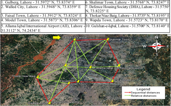
LOGISTICS The case study consists of 10 distinct locations of Lahore. Let’s assume Daraz courier have to visit these locations to deliver the packages to the customers. The satellite view of the selected areas of Lahore is shown in Figure 1. Here is the list of areas along with their coordinates that were selected to carry out this problem in which a delivery man was assumed to deliver the packages in following areas.
Figure 1: Satellite view map of the selected areas of Lahore.
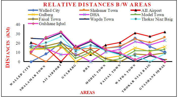
Each node must be visited only once in a round trip, aiming to minimize the total travel distance. The journey starts from Walled City and ends at Gulshan-e-Iqbal, with urban distances, not aerial ones, calculated via Google Earth. These distances, represented by red and green arrows, are shown in Table 1, while Figure 2 presents a graphical view of relative distances across selected areas of Lahore.
The problem is solved by the popular software tool like Excel. At first, the model is designed in Excel and after that the problem is solved by the optimization tool Solver Add-in, which is application software of Excel.
Table 1: Ground based distances between areas (in kilometers).
Application of the Travelling Salesman Problem in Optimizing Logistic Routes 149
Figure 2: Graph showing relative distances between the areas.
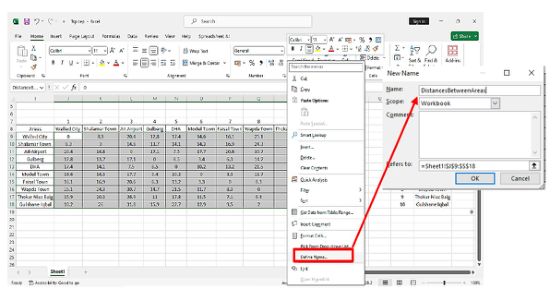
The whole procedure of solving this problem on excel is recorded as shown in following steps: Step 1: Defining the name of the Distances range. Firstly, selected the cell range of the distances (J9:S10) and defined its name “Distances Between Areas” as shown in the Figure 3.
Figure 3: Assigning name to the data of distances among areas.
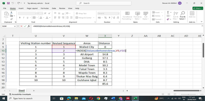
Step 2: Each area is assigned a visiting station number in Column U (U9:U19), revised based on the solver’s optimal sequence in Column V (V9:V19). The unknown variables are the revised visit sequence, determined using the INDEX function to extract objective function values from specified rows and columns. This function helps compute distances between route vertices, using initial parameters like data area and position indices. Apply “INDEX” formula on named range which is shown in Figure 4. In form “=INDEX(DistanceBetweenAreas, Location 1, Location 2)” will give us the distance from the previous visited area.
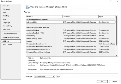
Step 3: Now in order to have Solver Add-in option, Select “File > Options > Solver-In” marked the solver-In from the list and clicked on “Go” as described in Figure 5.
Figure 4: Final model to be optimized.Figure 5: Adding solver add-in in excel.
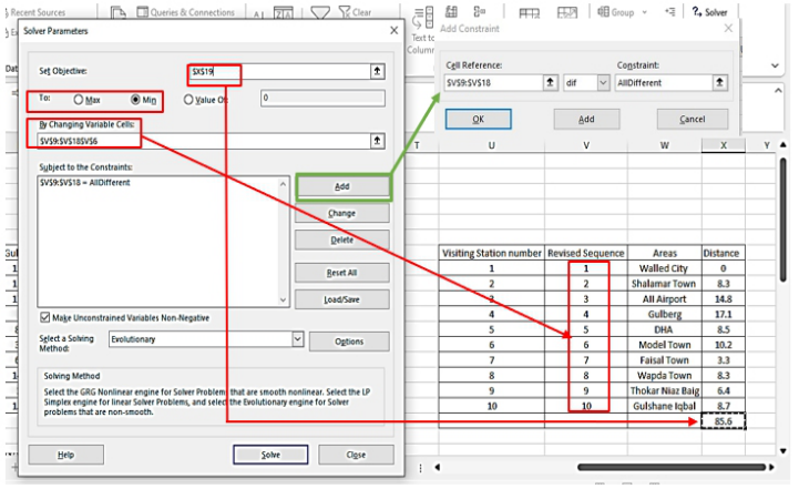
Step 4: Navigate through “Data” Tab and click on “Solver” located on extreme right of screen, a window will appear as shown following: Step 5: Set the total distance (X19) in “Set Objective” to minimize it, with changing variable cells as the area sequence (V9:V19). Use the evolutionary solving method, add constraints, and apply the “AllDifferent” function for optimization.
Step 6: After setting all of the variable click on “Solve” option. It will take some time and show results in reduced distance which you set as objective earlier.
Following table is showing the resulted sequence of visiting.
Application of the Travelling Salesman Problem in Optimizing Logistic Routes 151
Figure 6: Navigating solver window.Figure 7: Plugging values of solver parameters.Table 2: Sequence of visiting areas with minimial distance.
Table available in the original PDF paper.
Visiting Station
Revised Sequence Areas Distance Number 1 2 Walled City 0 2 1 Shalamar Town 8.3 3 10 All Airport 10.2 4 8 Gulberg 2 5 9 DHA 6.4 6 7 Model Town 7.1 7 6 Faisal Town 3.3 8 4 Wapda Town 3.4 9 5 Thokar Niaz Baig 8.5 10 3 Gulshane Iqbal 7.5 Total Distance 56.7 km
Now in order to check the cost of these Let’s take the example of Daraz Express The fuel average of Suzuki Bolan used by the Daraz Express is approx. 12.5 km/liter to delivering the packages from wear-houses of stores to Daraz Stores.
Current Price of Petrol: Rs. 256/- (As per rates on 16th January, 2025) Total cost before optimization= 85.6 km
Equation reproduced from the original PDF.Equation reproduced from the original PDF.
12.5 km X Rs. 256/- = Rs. 1162/- Difference in Cost 1753–1162 = Rs. 591/- The fuel average of a CD 70 Bike used by Daraz couriers to deliver the packages from Daraz store to customers is approx. 50km/liter.
Total cost of fuel before optimization = Rs. 439/- Total cost of fuel After devising Optimum path = Rs. 291/- Difference in Cost 439–291 = Rs. 148/- So, it concluded that daraz can save up to 34% of its cost using Suzuki Bolan and CD 70 Bike service by the utilization of Travelling Salesman problem.
TRANSPORTATION ROUTING
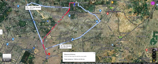
Figure 8: Speedo bus FR-04 satellite view (red line).
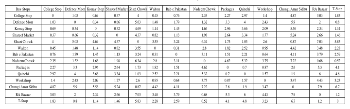
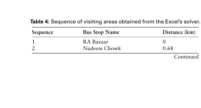
Another problem was implemented in terms of Speedo Bus Feeder Route 04 bus stops are randomly sequenced to check for the optimized and shorter route. Following are the relative Distances between Bus Stops (kms). Proposed & Actual Route after solving the TSP using Solver Add in, in the Excel is shown below in Table 4 and Table 5.
Table 3: Relative distance between each bus stop.Table 4: Sequence of visiting areas obtained from the Excel’s solver.
Application of the Travelling Salesman Problem in Optimizing Logistic Routes 153
Table 4: Continued Sequence Bus Stop Name Distance (km)
Table 5: Actual sequence of visiting areas of route 04 of speedo bus.
Table available in the original PDF paper.
Sequence Bus Stop Name Distance (km) 1 RA Bazaar 0 2 Nadeem Chowk 0.68 3 T-Stop 0.52 4 Defence Morr 0.8 5 Korray Stop 0.34 6 Shareef Market 0.32 7 College Stop 0.37 8 Walton 0.45 9 Bab e Pakistan 0.31 10 Workshop 0.64 11 Packages 0.87 12 Qainchi 0.7 13 Ghazi Chowk 1.03 14 Chungi Amar Sidhu 0.87
Total 7.9
The actual length of this Feeder route from RA Bazaar to Chunghi Amar Sidhu is approximately 8km (Adda and Store n.d.) & the obtained results are same as Table 4 the actual route of the bus illustrating optimized route of bus.
CONCLUSION
The successful implementation of the Travelling Salesman Problem (TSP) has resulted in significant advancements in mobility aspects. By optimizing routes, TSP enhances delivery efficiency, reducing travel time by determining the best sequence and location of delivery points. This ensures streamlined routes, minimizing detours and idling, which in turn lowers fuel consumption, supports environmental conservation, and cuts costs. Improved routing also boosts customer satisfaction by ensuring timely deliveries, fostering trust and loyalty. Efficient resource use reduces vehicle wear and fuel expenses, enhancing sustainability. Additionally, TSP reduces operational costs by minimizing mileage and optimizing stops, leading to
lower maintenance, fuel, and labor expenses, ensuring financial efficiency for transport companies.
REFERENCES
Adda, Lari, and Cooper Store. “No. of Buses Required.” (17): 14–17. Book, Ronald V. 1980. “Book Review: Computers and Intractability: A Guide to the Theory of $NP$-Completeness.” Bulletin of the American Mathematical Society. doi: 10.1090/s0273-0979-1980-14848-x. Dahiya, Chetna, and Shabnam Sangwan. 2018. “Literature Review on Travelling
Salesman Problem.” International Journal of Research. Kiunsi, Robert B. 2013. “A Review of Traffic Congestion in Dar Es Salaam City from the Physical Planning Perspective.” Journal of Sustainable Development. doi: 10.5539/jsd.v6n2p94. Lawler, E. L., J. K. Lenstra, A. H. G. Rinnooy Kan, and D. B. Shmoys. 1986. “The
Traveling Salesman Problem: A Guided Tour of Combinatorial Optimization.” The Journal of the Operational Research Society. doi: 10.2307/2582681. Meindl, S. Chopra and P. 2001. Supply Chain Management. 6th ed. New Jersey: Chopra, S., Meindl, P. Pekár, Juraj, Ivan Brezina, Jaroslav Kultan, Iryna Ushakova, and Oleksandr
Dorokhov. 2020. “Computer Tools for Solving the Traveling Salesman Problem.” Development Management. doi: 10.21511/dm.18(1).2020.03. Prokudin, Georgii, Olexiy Chupaylenko, Olexiy Dudnik, Alena Dudnik, and Yuriy Pylypenko. 2018. “Traveling Salesman Problem in the Function of Freight Transport Optimization.” Journal of Sustainable Development of Transport and Logistics. doi: 10.14254/jsdtl.2018.3–1.3. Prokudin, Georgiy, Olexiy Chupaylenko, Olexiy Prokudin, Olexiy Dudnik, and
Yuriy Pylypenko. 2018. “Optimization of transport processes with the use of information technologies .” European Journal of Intelligent Transportation Systems: 15–17. doi: 10.31435/rsglobal_ejits/30112018/6217. Ratliff, H. Donald, and Arnon S. Rosenthal. 1983. “Order-picking in a rectangular warehouse: A solvable case of the traveling salesman problem .” Operations Research. doi: 10.1287/opre.31.3.507. Stoilova, K., and T. Stoilov. 2020. “Transportation Modelling and Solving Travelling
Salesman Problem.” In IOP Conference Series: Materials Science and Engineering, doi: 10.1088/1757-899X/878/1/012026. Vukmirovi´c, Slavomir, and Drago Pupavac. 2013. Interdisciplinary Management Research The travelling salesman problem in the function of transport network optimalization .
LISTED IN THE AHFE DIGITAL BOOKSTORE CATALOGUE
Explore the complete digital volume
Creativity, Innovation and Entrepreneurship
Read this individual research paper free through the original publisher, or explore the full digital proceedings book.
ISBN 978-1-964867-42-7
Explore this ISBN in the AHFE Bookstore ↗Listed in the July 2026 bookstore catalogue; search by ISBN to confirm current availability · Digital book purchase optional