Sergey Pryalov, Vadim Seleznev (2020). Special Computational Gas Flow Simulation Methods for Trunkline Network Failures. In: Advances in Applied Digital Human Modeling. AHFE Open Access, vol. 11. https://doi.org/10.54941/ahfe100416
We consider two new methods for numerical solution of a complete system of partial differential equations describing the flow of a gas mixture in pipeline systems. The first method tracks Lagrangian particles as they move together with the flow of transported fluid. When implementing this method, the flow parameters are found by means of a difference scheme, and the distribution of mass fractions of components and enthalpy of matter along the pipeline, by analyzing the motion of the Lagrangian particles. If we ignore the processes of diffusion, these particles must preserve their composition. The energy equation without diffusion and heat conduction reduces to an ordinary differential equation. The method proposed is free of artificial viscosity, because, for example, when considering the equation of continuity of components, variations in their specific mass fractions at any point in space are related only to physically meaningful processes, namely, to the inflow of “new” particles (with “new" specific mass fractions of the components). The second method includes constructing spline functions along the space and time coordinates of the computational mesh subject to the fulfillment of differential equations at its nodes. The use of splines of high orders of approximation improves the accuracy of modeling.
Publications [1–4] propose industry-oriented approaches to numerical modeling of operating conditions of complex trunkline networks that transport process gases, liquids and multiphase fluids. These publications repeatedly pointed at the necessity of improving the accuracy of simulations using the mathematical models proposed, first of all, to enable credible simulation-aided failure analysis. As we know, one of the central accuracy improvement prerequisites is a science-based choice of appropriate techniques for the numerical analysis of the mathematical models developed. The present paper discusses current versions of two efficient techniques of numerical analysis of mathematical gas flow models for trunkline failure analysis. They have demonstrated their efficiency in practice as applied to failure analysis of gas distribution networks of Gazprom’s subsidiaries.
DESCRIPTION OF THE FIRST NUMERICAL ANALYSIS METHOD FOR MATHEMATICAL MODELS OF GAS FLOW IN TRUNKLINE NETWORKS Let natural gas, which in the first approximation can be treated as a single-component gas with known physical and mechanical properties, be transported through a network of branched pipelines with absolutely stiff rough heat conducting walls.
To solve the problem, we use the following computational approach: we conventionally assume that each supplier (in our case, “supplier” refers to a dispatching control station) introduces a unique grade of a single-component chemically inert gas, the properties of which are exactly the same as those of natural gas, to the common collector. In this case, as a result of non-isothermal mixing in the common collector and downstream pipelines, a multi-grade homogeneous chemically inert gas mixture will form, possessing physical and mechanical properties of the initially transported natural gas. Its grade (or component) composition will vary with time only due to corresponding variations in the gas supply conditions and parameters of gas consumption from the given pipeline system.
Based on the time variations of the gas mixture composition at the outlet boundary of the downstream pipeline associated with a certain consumer, one can conclude, which particular suppliers influence the volume of gas supply to the given consumer. Constructing the target functions of gas grade shares versus time reduces to numerical modeling of non-steady-state non-isothermal homogeneous multi-component time-variant-composition gas mixture transport through the given gas distribution network of long branched pipelines. Here, considering the natural gas flow velocities in common collectors and downstream pipelines, one can ignore the influence of diffusion and heat conductivity in the gas flow direction without loss of accuracy of simulation results [4].
One of the most promising approaches to credible numerical evaluation of space-time distribution of physical flow parameters in pipeline systems involves using the high-accuracy computer gas dynamic simulator to model the performance of the system of interest (GDS) [1, 4]. The gas dynamics model of non-steady-state non-isothermal turbulent flow (without diffusion and heat conductivity along the gas flow) of a multi-component homogeneous mixture of viscous chemically inert compressible gases through a branched system of long varied round cross- section graded pipelines with absolutely stiff rough heat conducting walls, as implemented in the computational core of GDS, can be represented as follows: – for each pipe (bend or non-branched segment of the common collector):
(1)
(2)
(3)
(4)
– for each junction (boundary sections of pipelines adjoining the junction):
(5)
(6)
(7)
(8)
(9)
(10) (11)
(12)
– equations of state [5]:
(13)
(14)
where is the gas mixture density; is the pipeline flow section area; is the time (marching variable); is the spatial coordinate along the pipeline axis; is the projection of the vector of gas velocity averaged over the pipeline cross section to the pipeline axis (on the assumption of developed flow turbulence); is the mass
fraction of the -th component; is the reduced density of the -th component (mass of the -th component in unit volume of the mixture); is the number of mixture components; is the static gas mixture pressure;
is the gravity acceleration modulus; is the spatial coordinate of the point in the pipeline axis reckoned from an arbitrary horizontal plane vertically upward (for trunklines, along the Earth radius); is the Pythagorean number; is the hydraulic friction coefficient in the Darcy–Weisbach formula; is the inner pipe radius; is
specific (per unit mass) enthalpy of the mixture; is specific (per unit volume) power of heat sources; is the gas mixture temperature; is the number of pipes constituting the given junction; is the subset of upstream pipes of the given junction (upstream pipes with respect to the junction are the pipes, through which the gas enters
the junction); is the subset of downstream pipes of the given junction (downstream pipes with respect to the junction are the pipes, through which the gas leaves the junction); is the static gas mixture pressure in the
given pipeline junction; is the gas mixture temperature in the pipeline junction (i.e. in the inner space of the junction); is the mass fraction of the -th gas mixture component in the junction; is the specific (per
unit mass) enthalpy of the gas mixture in the junction of interest. The function characterizes the heat exchange of the gas flow core through the boundary gas layer, pipe wall and insulation with the environment. It expresses the total specific (per unit length) thermal flux along the perimeter of the cross section having an area
of from the transported gas to the environment (
means heat removal; is the space-time
distribution of ambient temperature at the domain boundary). To indicate that a quantity belongs to the -th pipe, we use a superscript in parentheses left of the quantity, for example: . The system of equations (1–14) is supplemented with boundary conditions and conjugation conditions. As conjugation conditions we can define boundary conditions simulating a complete rupture of the pipeline and/or its shutoff, operation of valves, etc.
To numerically solve the system of equations (1–14), the computational core of GDS usually employs grid methods. Unfortunately, distribution trunkline networks contain a large number of pipe joints distributed on general collectors extremely nonuniformly. In our case, this results in the necessity of considerable spatial mesh refinement and, consequently, in a much longer runtime. Such an increase in the runtime is intolerable in simulations done to provide computer-aided support of pipeline dipatcher decisions.
To overcome this situation, the computational core of GDS employs a hybrid modification of the known integro- interpolation method developed by A. N. Tikhonov and A.A. Samarsky [6, 7] and S.N. Pryalov’s Lagrangian particle method [4]. The Lagrangian particle method is applied only to the equations of component continuity (2, 5, 7) and energy equations (4, 6, 7). Note that this Lagrangian particle method is essentially a dedicated modification of the approach for solving hyperbolic partial differential equations by the well-known method of characteristics [8]. Let us consider the algorithm of applying this method to the component continuity equations.
As we know, in a non-steady-state flow of a gas mixture through a branched network system, regions (moving together with the gas flow) can occur, where concentrations of the mixture components can differ significantly from those in neighbor regions. The use of difference schemes may lead to substantial front “smearing”. Given that the difference schemes [6, 7] are conservative, the total mass of the mixture components in the pipeline network will not vary with time. However, the values of component concentrations can decrease (or increase) unreasonably, and as a result, the fluid of these materials will get non-physically “smeared” along the length of the pipeline. The idea of the Lagrangian particle method in this case rests upon the known fact that if we separate a small particle of matter (a small moving volume of matter), the continuity equations of the components will actually describe the motion of this particle (with some set of components) with the gas flow. Accordingly, it is suggested that the component continuity equation be solved by analyzing the motion of some set of particles in the gas flow. Flow parameters in this case can be defined in any manner enabling simulation of a single-component gas flow (for example, by finite differences). Owing to the way of introducing these particles, they are conventionally called Lagrangian.
The general algorithm of flow modeling without multicomponent gas mixture diffusion in branched pipeline systems using the Lagrangian particle method can be described as follows (S.N. Pryalov’s algorithm):
1. Initially, along the length of every -th pipeline we “place” a set of Lagrangian particles ordered by increasing coordinates (with numbering ) in the amount of at a distance on the order of the length of a spatial mesh cell. A mandatory requirement is that the Lagrangian particles with numbers
and lie on the left (coordinate ) and on the right (coordinate , where is the length of the -th pipeline) pipeline boundaries, respectively. Specific fractions of the
components for the particles are defined by approximation of initial conditions. Let be the coordinate of the -th Lagrangian particle belonging to the -th pipeline for the -th time step.
2. Gas dynamic variables of the gas mixture flow at the next time step are calculated (using difference equations approximating the gas dynamics equations (1–14), except for the component continuity equations (2, 5, 7) and energy equations (4, 6, 7)). The values of the specific component fractions at mesh nodes are defined by interpolation between these values for the Lagrangian particles adjacent to the mesh node.
3. For each -th Lagrangian particle of each -th pipeline, we update the coordinate for the new time step using the formula:
(15)
4. For each pipeline, we delete the Lagrangian particles that leave the pipeline. At the same time, a new particle is generated at the corresponding “outlet” boundary (the boundary, through which the gas leaves the pipe) with specific component fractions equal to the interpolated values of the particles closest to the boundary: inside the pipe and outside the pipe (the latter particle is deleted with respect to the pipe).
5. For each pipeline junction, specific component fractions are calculated by the following formula: (16)
where is the specific mass fraction of the -th component of the particle located at the outlet boundary of the upstream pipeline; , and are the gas mixture density, velocity and cross section area corresponding to the outlet boundary of the upstream pipeline. 6. For each inlet boundary of each pipeline, a new Lagrangian particle is generated with specific component fractions corresponding to the boundary conditions (if the boundary is inlet for the given pipeline system) or equal to the specific component fractions in the pipeline junction (if the boundary adjoins the junction). At the next time step, if the distance between this particle and the following (downstream) particle is smaller than the given distance (on the order of the spatial cell length), this particle is deleted.
7. If reaches the limiting value, the simulation is completed. Otherwise, we assume that and proceed to step 2.
Since the Lagrangian particle method for the energy equation is not related directly to the finite difference mesh employed for solving the continuity and motion equations, this mesh has almost no effect on the accuracy of the proposed method. Thus, high-accuracy calculated values of gas temperature are obtained without mesh refinement, which speeds up the calculations significantly.
In addition, due to the absence of direct connection between the Lagrangian particle method and the finite difference mesh, this method is free of the so-called artificial viscosity (see above and [6, 7]). As a result, the method makes it possible to obtain solutions without artificial smoothing of temperature fronts, which corresponds to real physical processes. This significantly increases the credibility of simulations compared to the use of difference schemes for the energy equation.
DESCRIPTION OF THE SECOND NUMERICAL ANALYSIS METHOD FOR MATHEMATICAL MODELS OF GAS FLOW IN TRUNKLINE NETWORKS To improve the credibility of numerical modeling of trunkline network operation, it is reasonable to use conservative difference schemes.
This section of the paper considers an approach that uses fully conservative spline schemes for solving a complete system of gas dynamics equations for the case of a model describing the flow of a single-component gas in a trunkline. The consequence of (1–14) for an unbranched trunkline, considering the adopted assumptions, is the system of equations [4]:
(17)
(18)
(19)
(20) (21)
where is the specific (per unit mass) internal energy.
As we know, for systems of nonlinear partial differential equations (to which the system (17–21) belongs), in the general case, it is impossible to obtain an analytical solution. There exist various methods for constructing difference counterparts of original differential equations that enable obtaining difference equations possessing different properties. To produce a credible solution, the difference counterpart (the difference scheme) should be convergent [6, 7]. This property holds true if the difference scheme possesses approximation and robustness. In addition, the scheme should preferably be conservative and have an increased order of approximation (these properties allow the scheme to produce more accurate numerical solutions).
This section of the paper proposes employing spline schemes for solving a complete system of gas dynamics differential equations [4]. This method involves searching for target values of the gas dynamic parameters at the nodes of the space-time mesh such that the gas dynamic differential equations at the difference mesh nodes are satisfied, when approximating the distributions of these parameters by splines (along the space and time coordinates).
This method possesses an increased order of approximation; it is proven to be fully conservative, which provides higher credibility of process modeling when analyzing the parameters of gas transport in trunklines. On the other hand, spline schemes are implicit, which makes them more robust compared to explicit and semi-implicit schemes.
Let us begin considering this type of schemes from the simplest case, when splines are used to solve ordinary differential equations (see, e.g., [9]).
Let us discuss application of a spline scheme for solving the system (17–21). Let the spline order be with respect to the time coordinate and with respect to the spatial coordinate. The spline scheme for solving (1) can then be represented in the form proposed by S.N. Pryalov [4]:
(22a)
(22b)
(22c)
(22d)
(22e) The spline scheme (22) approximates a nondivergent form of mass, momentum and energy conservation laws (17– 21). The differential forms of these laws are satisfied at the nodes of the space-time mesh. Accordingly, the divergent forms of the principal conservation laws are also satisfied at the mesh nodes. If the spline order ensures the continuity and differentiability of the functions under the derivative sign in (17–21) (which requires that the conditions , hold), then there exists a divergent discrete counterpart for each divergent derivative. Consequently, the spline scheme is also conservative for systems of partial differential equations.
As the conservation laws are satisfied in the differential form at the mesh nodes, it follows that all possible representations of a given system are satisfied at these nodes (for example, equations for kinetic energy, total energy, entropy etc.). The existence of divergent discrete counterparts of all the divergent differential derivatives in this case ensures that the spline scheme is not only conservative but completely conservative [6, 7].
This conclusion is extended similarly to the continuum mechanics equations of any dimensionality. Thus, we show that a spline scheme is completely conservative. This enables modeling gas and hydrodynamics processes with higher credibility and accuracy due to the correct modeling of all possible conservation laws. On the other hand, spline schemes are implicit, which makes them more robust compared to explicit and semi-implicit schemes [6, 7]. Increasing the order of the splines used makes it possible to increase the order of approximation of gas- and hydrodynamic equations, which also improves the accuracy of simulations.
EXAMPLES OF PRODUCTION SIMULATIONS Efficiency of the method of numerical recovery of gas flows in trunkline systems proposed in the paper was demonstrated in 2010–2014 in production simulations at GAZPROM Mezhregiongaz Moscow LLC within the Alfargus/Mosregiongaz Computer System (Fig. 1).
Figure 1. Example of the Alfargus/Mosregiongaz Computer System application in the control room of GAZPROM
Mezhregiongaz Moscow LLC
The method was used for numerical recovery of the flow of natural gas delivered (from a single supplier) to consumers through seven branches of the Moscow Gas Ring (MGR). MGR has a total length of over 200 km and more than 130 consumer branches. The flow was recovered at 106 IPs, which were relatively uniformly distributed over the gas pipeline ring.
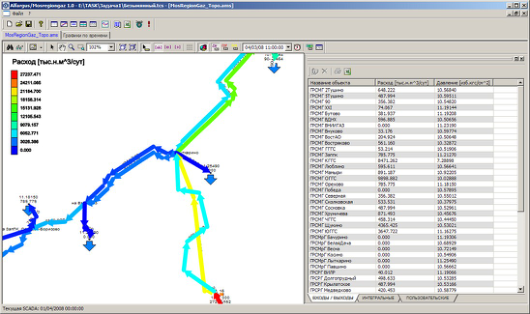
The transport flow is transient nonisothermal gas flow. The example of flow diagram (i.e. recovered flow direction and numerical estimates of volumetric flow rate of natural gas [dimension: thousand cubic meters per day] in accordance with color gradation) in the South-East MRG sector (temporal section) was shown on Fig. 2. In table on the right of Fig. 2 one can see quantitative estimates of gas flow rate distribution [column 2, dimension: thousand standard cubic meters per day] and gas pressure [column 3, dimension: gauge atmospheres] for recovered flows in specific branches in the South-East MRG sector (temporal section). In the first column of the table under consideration description of branches are given in topographical map reference.
The example of diagram correlation of time history of calculated and measured estimates of pressure and mass flow rates for one from the IPs, which is used in MGR (gas flow temperature was measured with a poor accuracy and long time intervals and was not suitable for comparative analysis) was shown on Fig. 3. It should be noted that measurement results underwent preliminary verification and smoothing. The recovered gas flow parameters were used to analyze the performance of MGR, and to detect and localize the sources of discrepancy in estimated volumes of gas supply through MGR.
Earlier versions of the flow recovery method were used to investigate trunkline accidents and to train gas pipeline operators in efficient pipeline control under conditions as close as possible to real operation of gas transmission and delivery systems using high-accuracy computer simulators.
Figure 2. Example of flow diagram in the South-East MRG sector (temporal section)
a) b) Figure 3: Example of curve correlation of calculated and measured pressure history (a) and mass flow rate (b) for one from the
IPs used in MGR
CONCLUSIONS
In 2008–2014 these methods demonstrated their efficiency as applied to production simulations done to validate discrepancy mechanisms in natural gas supply through the Moscow circular gas trunkline. Application of these methods in practice does not require any special high-performance computers.
REFERENCES
Ahmed T.H. (2007), “Equations of State and PVT Analysis: Applications for Improved Reservoir Modeling”. Gulf Publishing Company, Houston. Fletcher С.A.J. (1988), “Computational Techniques for Fluid Dynamics: Fundamental and General Techniques”. Springer-
Verlag, Berlin. Ortega J.M., Pool W.G. (1981), “An Introduction to Numerical Methods for Differential Equations”. Pitman Publishing Inc. Seleznev V.E. (2007), “Numerical simulation of a gas pipeline network using computational fluid dynamics simulators”. Journal of Zhejiang University SCIENCE A. Vol. 8. No. 5. P.755–765. Seleznev V.E., Pryalov S.N. (2011), “Gas-Liquid Flow Model for Branched Trunklines”. Applied Mathematical Sciences. Vol. 5,
No. 65. PP. 3233–3261. Seleznev V.E. (2012), “Numerical Recovery of Gas Flows in Pipeline Systems”. Journal of Applied Mathematics. Vol. 2012.
Article ID 180645. 25 p. Seleznev V.E., Pryalov S.N. (2014), “Computational Fluid Dynamics of Trunkline Systems: Methods for Constructing Flow Models in Branched Trunklines and Open Channels”. M.: KRASAND. Samarsky A.A., Popov Yu.P. (1992), “Difference Schemes for Solving Gas Dynamics Problems”. Moscow, Nauka. Tikhonov A.N., Samarsky A.A. (1999), “Equations of Mathematical Physics”. Moscow, MSU Publishing Office.
LISTED IN THE AHFE DIGITAL BOOKSTORE CATALOGUE
Explore the complete digital volume
Advances in Applied Digital Human Modeling
Read this individual research paper free through the original publisher, or explore the full digital proceedings book.
ISBN 978-1-4951-2094-7
Explore this ISBN in the AHFE Bookstore ↗Listed in the July 2026 bookstore catalogue; search by ISBN to confirm current availability · Digital book purchase optional