Wenjuan Zhang, Xiujie Li, Bin Zhang, Haozhe Yang, Guangbin Wang (2023). Short-time taxi demand prediction based on Transformer-LSTM in integrated transportation hub. In: Human Factors in Software and Systems Engineering. AHFE Open Access, vol. 94, pp. 54–63. https://doi.org/10.54941/ahfe1003770
Taxis, as an important part of the comprehensive transportation passenger flow connection, is one of the main tools for passengers in an integrated transportation hubs due to their better accessibility and convenience. Due to the impact of passenger travel choices and the frequent collection and distribution of large passenger flows in comprehensive transportation hubs, the demand for taxis fluctuates greatly. In addition, there are many other uncertainties in the process of taxi transfer because of the unreasonable scheduling of taxis, such as long transfer time, passengers stranded at the taxi stand, etc. Thus will cause delay and time waste of passengers. In order to improve the productivity of the hub operation in passenger flow distribution and serve the dynamic decision-making of taxi drivers, it is very necessary to predict the demand for taxis in the hub in time. Based on artificial intelligence deep learning method, this paper wants to build a short-term taxi demand forecasting model, which can assist taxi drivers to make decisions and choose a reasonable time to wait go to the taxi storage yard, so as to match the taxi demand of passengers with the supply of taxis perfectly and reduce the waiting time. By learning to fully mine the time-series characteristics of the historical data of taxis flow, the model integrates the Transformer and the LSTM neural network for the short-term prediction of demand of taxis every 15 minutes. Then taking the Shanghai Hongqiao transportation hub as an example, the experiment collected 3months of taxi cross-section traffic data to train the model. The results shows that the trained Transformer-LSTM model has a high accuracy in predicting short-term taxi demand. In order to verify the superiority of the model, the designed model is compared with other prediction models, such as CNN, LSTM. The experimental results show that the comprehensive performance of the Transformer-LSTM model has the highest accuracy. The model can be used to provide a forecast service for passengers' demand for taxis in transportation hubs, and provide a powerful reference for the optimization of taxi dispatching.
With the rapid development of transportation modes, passenger flow in large transportation hubs is increasing year by year, which poses challenge to hub’s operational capacity. Inconvenient interchange methods affect passengers’ satisfaction largely, and many passengers stranded in the hubs can also be a safety hazard (Zhong et al. 2020). As one of the main modes of transfer- ring within the hub, taxis scheduling still have many problems, such as long transfer times and long queues of waiting. Therefore, basing data to forecast the demand for taxis in the hub is necessary. Traffic data contains characte- ristics of passenger flow, using intelligent algorithms to deep mine the data can provide powerful and efficient on passenger flow prediction.
Transportation related forecasting has been studied for a long time, such as airport passenger flow forecasting (Lin et al. 2022) and taxi demand
Short-Time Taxi Demand Prediction Based on Transformer-LSTM 55
forecasting (Rodrigues et al. 2019). Traditional methods for traffic predi- ction include ARIMA models (Chen et al.2019) and Kalman filters(Jiao et al. 2016). With the development and application of traffic big data, more and more scholars’ research moves to deep learning methods, such as the com- monly used improved RNN, including LSTM (Han et al. 2019; Wang et al. 2020), GRU (Yang et al. 2019), and CNN in combination with other meth- ods(Liu et al. 2020). These researches contribute great value to hub taxi demand forecasting, but most models ignore the importance of short-time forecasting and data periodicity features, which leads to insufficient accu- racy and timeliness of the forecast. This paper tries to propose a combined deep learning short-time prediction model combining LSTM neural network and Transformer, to process time series data and fully exploiting the time periodicity features.
PROBLEM DESCRITIONS This paper focuses on taxi demand forecasting in large transportation hubs. The paper takes the historical data of taxi departures from the storage yards in the past, and forecasts the departures in the future period. The mathe- matical description of the problem is as follows: at a given time step t, the sequence HT1={yt−T1−1, yt−T1, .., yt}of the previous T1 steps of the historical data is used to predict the sequence HT2={yt + 1, yt + 2, .., yt + T2} correspon- ding to the next time step T2. T1 denotes the input step of the prediction model, T2 denotes the output step of the prediction model, and yi denotes the historical departure volume for time step i.
Suppose D={y1, y2, .., yn} is denoted as a time series of length n time steps, then before model prediction, it is also necessary to reconstruct the sequence D in the form of HT1, HT2with a sliding window, T1 for an input step of and an output step of T2, the sliding window is T1+T2, i.e., for each sliding one unit, it produces n-T1 sequences of length T1+T2, where the first T1 data of each sequence are used as input Xi and the last T2 data are used as output Yi. After data reconstruction, the input set of the model is Xin={X1, X2, . . . , Xj}, and the output set is denoted as Yout={Y1, Y2, . . . , Yj}.
We focuses on the single-step prediction problem, i.e., T2 = 1, using data from the past T1 time steps to predict data from the next time step, so the pivotal taxi prediction problem defined in this paper can be expressed by the following equation: Yt = G((Xt−T1, . . . , Xt−1)) (1)
where, G(·) denotes the mapping function, Yt is the model prediction at time step t, and (Xt−T1, . . . , Xt−1) denotes the sequence of the past T1 time steps.
METHODS
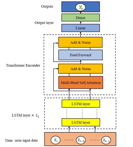
This paper proposes a combined deep learning prediction model, namely the Transformer-LSTM model, which mainly contains two parts, the first part is LSTM neural network layer, and the second part is the improved Transformer encoder. The structure of the model is shown in Fig. 1.
Figure 1: Model structure.
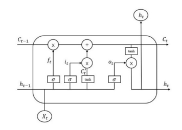
LSTM NEURAL NETWORK LAYERS Due to the poor performance of RNN in long sequences, Hochreiter (Hoch- reiter et al. 1997) proposed LSTM neural network, which is a special type of RNN that introduces “cell” in the structure to record additional informa- tion. We use LSTM neural network to mine the continuity features of the input time series. The structure of the LSTM unit is shown in Fig. 2.
In Fig. 2, xt denotes the input at time step t and ht denotes the output at time step t. The formulas for the whole structure are as follows.
Equations and mathematical formulas are available in the original paper PDF.
ht−1, xt
Wf ·
Equations and mathematical formulas are available in the original paper PDF.
Wi ·
+ bi
ht−1, xt
Figure 2: LSTM unit structure.
Short-Time Taxi Demand Prediction Based on Transformer-LSTM 57
ht−1, xt
WC ·
+ bC
Equations and mathematical formulas are available in the original paper PDF.
Wo ·
+ bo
where σ(·) is the sigmoid activation function with the output range [0,1]; tanh(·) is the hyperbolic tangent activation function; Wf, Wi, WC, Wo are the weight matrices; bf, bi, bC, bo are the bias terms.
The number of LSTM combinatorial model layer is L1, the number of hidden layers by each LSTM layer is 64, and the output features are set to 10. Assuming an input step size of d, the LSTM layer outputs a (10 × d) matrix, which is represented as the result of learning continuity features from the LSTM layer.
TRANSFORMER LAYERS In the prediction of time series, the input and output are continuous, and there is no semantic position correspondence, so this paper discards the position encoding method and directly concatenate with the LSTM layer mentioned above to make up for the shortcomings of transformer in extracting temporal features. In this layer, the encoder part of the original Transformer model is retained, and the encoder includes the feed-forward network layer and the self-Attention layer; the model discards the mask operation of the encoder and uses the multi-headed self-attention mechanism to mine the temporal features, and finally outputs the results through the linear layer.
MULTI-HEAD SELF-ATTENTION MECHANISM Vaswani (Vaswani et al. 2017) proposed the Transformer model in 2017, which uses the self-attention structure instead of the RNN structure com- monly used in NLP tasks, and its biggest advantage over the RNN network structure is that it allows for parallel computation.
In this paper, the self-attention mechanism is used to calculate the corre- lation between time steps in the taxi flow input matrix X by three vectors: Query(Q), Key(K) and Value(V). The input matrix X of the Transformer layer, which is also the output matrix of the LSTM layer, is a (10 × d) matrix. The calculation formulas are as follows: Q = XWQ, Q ∈R10×d (8)
!
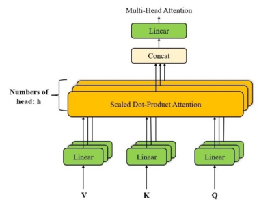
Figure 3: Multi-head self-attention mechanism.
Where WQ, WK and WV are weight matrices; dK is the vector dimension of matrix K; S ∈R10×d is the similarity matrix between Q and K; Z is the output of the self-attention mechanism.
In addition, we introduce the multi-head self-attention mechanism to use each set of attention to map the input to a different sub-representation space, which allows the model to exploit the periodicity features of the taxi flow more adequately. The structure of the multi-head self-attention mechanism is shown in the Fig. 3.
In the model, h self-attention heads are set to be computed in parallel. The output of each self-attention head is stitched horizontally in the computation process to obtain a (10×d×h) matrix, which is multiplied with the mapping matrix to obtain. The mapping matrix can fuse all the traffic timing infor- mation, and the output matrix has the same dimension as the input matrix, which can contain the output information of each self-attention head. The calculation formula is as follows.
ZM = Contact(Z1, Z2, . . . , Zi, . . . , Zh)WO (13) Where Contact(·) is the matrix splicing function; Zi denotes the output of the i th self-attended header; WO ∈R[d×h]×d is the mapping matrix.
DATA DESCRIPTION AND PRE-PROCESSING The dataset used in this paper is from the North Taxi Storage Yard at Hong- qiao High-Speed Railway Station, Hongqiao Hub, Shanghai. The dataset describes the daily taxi departures of the North Storage Yard at a granu- larity of 3 minutes, and the data from 8:00-24:00 per day from January 1, 2021, to June 31, 2021, at the North Storage Yard are selected for this expe- riment. To meet the requirement of real-time prediction, the experiment was divided into 96-time steps per day with a granularity of 15 minutes. In terms of pre-processing, the data need to be normalized before being input to the model, and this paper uses the Max-min method to deflate the data to the [0, 1] interval, and the formula for the normalization of Max-min is shown
Short-Time Taxi Demand Prediction Based on Transformer-LSTM 59
in (14).
Where Xnorm denotes the normalized value, Xmax denotes the maximum value of the data, Xmin denotes the minimum value of the data, and X denotes the original value. Finally, the preprocessed data are divided into a training set Train_data, a testing set Test_data, which are used for model training and validation respectively.
MODEL EVALUATION METRICS The time series forecasting model is a regression model, so the two evalua- tion indicators, MAE (Mean Absolute Error) and RMSE(Root Mean Square Error), are chosen to evaluate the forecasting performance of each model. MAE can be used to assess the similarity between the predicted and true values, and the smaller the mean absolute value error, the better the model fits the data; RMSE indicates the sample standard deviation of the devia- tion between the predicted and true values. The two evaluation indicators are calculated as follows.
m X (|yi −ypre|) (15)
(ypre −yi)2 (16)
Where yi is the true value of the i th test sample, ypre is the predicted value of the i th test sample, and m is denoted as the number of test samples.
MODEL ENVIRONMENT The experimental model development environment is GPU: NVIDIA GeForce GTX 1050 Ti, memory RAM: 8GB, system: Windows 10, language: Python 3.7, IDE: Anoconda3 spyder. the model is built based on the deep learning framework Pytorch, while setting the model’s batch_size The model is built based on the deep learning framework Pytorch, and the model’s batch_size is set to 32, the model loss function is MSE, the learning rate is 0.005, the optimizer is selected as Adam, and the activation functions are all ReLU functions.
MODEL PARAMETER TUNING The model parameters tuning session was conducted using the taxi north storage yard data for the input time step d, the number of LSTM layers, L1 the number of hidden layers n and the number of self-attention heads h. The range of each parameter was selected within a certain range of values: d=(2,4,6,8,10); n=(32,64,128); L1 =(1,2,3); h=(2,5,10). The experiments
of tuning use evaluation metrics MAPE( and RMSE to determine the effect of different parameter values on the prediction accuracy of the model. The tuning session uses the control single variable method, i.e., only one para- meter is adjusted at a time and the other parameters remain unchanged, and after finding the optimal value, the value is fixed and the tuning of the next parameter is carried out.
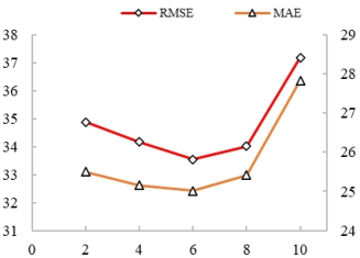
First, the input time step d is tuned. The results are obtained for each value of d=(2,4,6,8,10) by traversing the Table 1 and Fig. 4 from Table 1, the prediction error of the model is minimized when the input step d = 6.In Fig. 5, as d increases from 2 until 6, the error of the model keeps decreasing to 8 when the error is minimum, and as d exceeds 6 the error of the model gradually increases again. Therefore, the model performs best when the input step d = 8, and this parameter will be used in the next step for tuning the other parameters.
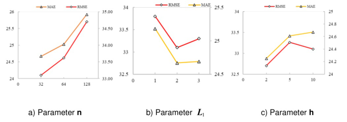
Next, the number of LSTM layers L1, the number of hidden neurons n, and the number of self-attention heads h are tuned as above. The experimental results are shown in Fig. 5 and Table 2.
From Table 2, we can see that for LSTM hidden layers n, the model has the best prediction effect when n=32 at the beginning, and the model accuracy keeps decreasing with the increase of n. Although theoretically increasing the number of hidden layers will improve the model effect, too many will lead to model overfitting and affect the model accuracy. For the number of LSTM layers L1, the model accuracy increases when L1 increasing from 1 to 2, but decreases when L1 increasing from 2 to 3, indicating that the number of LSTM layers L1 is sensitive to the model. Increasing or Decreasing one layer will significantly affect the model accuracy, so when L1=2, the model
Table 1. Results of parameter d tuning.
Table available in the original PDF paper.
Parameter MAE RMSE d 2 25.50 34.87 4 25.16 34.16 6 25.02 33.54 8 25.42 34.01 10 27.83 37.18
Figure 4: Results of parameter d tuning.
Short-Time Taxi Demand Prediction Based on Transformer-LSTM 61
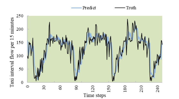
accuracy is the best. For the number of Transformer self-attention heads h, the model accuracy is the highest when h=2 at the beginning, and the model accuracy keeps decreasing as increasing to 5 and 10, indicating that the num- ber of self-attention heads has a great influence on the model prediction. Moreover, the number of self-attention heads needs to be divisible by out- put_size = 10 when setting, so the setting value can only be 2, 5 and 10, which has some limitations and affects the model accuracy. In conclusion, the optimal combination of parameters for the LSTM-Transformer model, i.e., d=6, n=32, L1=2, h=2, was finally determined, at which the evalua- tion metrics MAE = 24.25 and RMSE = 32.70 is at most 6.4% and 5.8% lower than the MAE and RMSE values of other parameter combinations. The Fig. 6 shows the prediction effect of the model for the first 250 time steps of the dataset. It can be seen that the model captures the temporal characteristics of the dataset well and has a good prediction effect.
MODEL PERFORMANCE COMPARISON To verify that the proposed Transformer-LSTM model has excellent per- formance, the dataset of the taxi north storage yard is selected for the experiments, and the obtained results are compared with GRU, CNN, and LSTM models. The experimental results are shown in Table 3.
From Table 3, it can be seen that the LSTM-Transformer model has the lowest MAE and the second lowest RMSE for the prediction of the dataset,
Figure 6: Part of predicted and actual results.Table 3. Model comparison results.
Table available in the original PDF paper.
Model name MAE RMSE LSTM-Transformer 24.25 32.70 CNN 32.61 39.23 GRU 24.78 31.73 LSTM 28.56 35.79
and the RMSE of the LSTM-Transformer model is 16.6% and 8.6% lower than the other two baseline models, CNN and LSTM, respectively, while the MAE is also 25.6% and 15.1% lower than them, respectively,which can indi- cate that the error between the prediction results of our proposed model and the true value is smaller, and the prediction accuracy is significantly impro- ved compared with other models. On the other hand, the experimental results show that GRU has the lowest RMSE and the second lowest MAE in terms of prediction accuracy. This shows that the LSTM-Transformer has very good accuracy in prediction on the dataset, and the LSTM-Transformer accuracy is similar to the GRU model. It is worth mentioning that GRU, as an excel- lent recurrent neural network for processing time series, has good accuracy in predicting regression problems.
CONCLUSION
To improve the operational management efficiency of transportation hubs, a combined model of taxi short-time prediction based on the LSTM neural network and Transformer model is proposed. Model comparison experi- ments were conducted using three baseline models, CNN, LSTM, and GRU, and the experimental results showed that the LSTM-Transformer model has
Short-Time Taxi Demand Prediction Based on Transformer-LSTM 63
good accuracy compared with other models, while the accuracy of the LSTM- Transformer model is similar to the GRU model. The demand for taxis is affected by other modes of transportation and external uncertainties out of the hub, and these problems are not considered in this paper. In the subsequent study, we will consider the influence of more factors and the traf- fic patterns of the hub to conduct a more in-depth study of taxi demand forecasting problem.
REFERENCES
Chen, E., Ye, Z., Wang, C., Xu, M., (2019). Subway Passenger Flow Prediction for Special Events Using Smart Card Data. IEEE Transactions on Intelligent Transportation Systems, 21, 1109–1120. Han, Y., Wang, C., Ren, Y., Wang, S., Zheng, H., Chen, G., (2019) Short-Term
Prediction of Bus Passenger Flow Based on a Hybrid Optimized LSTM Network. International Journal of Geo-Information, 8(9), 366. Hochreiter S., Schmidhuber J., (1997). Long short-term memory. Neural computation, 9(8), 1735–1780. Jiao, P., Li, R., Sun, T., Hou, Z., Lbrahim, A., (2016). Three revised Kalman filte-
ring models for short-term rail transit passenger flow prediction. Mathematical Problems in Engineering, 2016(3), 1–10. Lin, L., Liu, X., Liu, X., Zhang, T., Cao, Y., (2022). A prediction model to forecast passenger flow based on flight arrangement in airport terminals. Energy and Built Environment, S2666123322000423. Liu, T., Wu, W., Zhu, Y., Tong, W., (2020). Predicting taxi demands via an attention-
based convolutional recurrent neural network. Knowledge-Based Systems, 206, 106294. Rodrigues, F., Markou, I., Pereira, F. C., (2019) Combining time-series and textual data for taxi demand prediction in event areas: A deep learning approach. Information Fusion, 49, 120–129. Vaswani, A., Shazeer, N., Parmar, N., Uszkoreit, J., Jones, L., Gomez, A. N., Kaiser,
L., Polosukhin, I., (2017). Attention Is All You Need. arXiv. Wang, S., Zhao, J., Shao, C., Dong, C. D., Yin, C., (2020). Truck Traffic Flow Prediction Based on LSTM and GRU Methods With Sampled GPS Data. IEEE Access, 8, 208158-208169. Yang, D., Chen, K., Yang, M., Zhao, X., (2019). Urban rail transit passenger
flow forecast based on LSTM with enhanced long-term features. IET Intelligent Transport Systems, 13(10), 1475–1482. Zhong, M.and Liu, Y., (2020). Research on the Evaluation Index System of the Taxi Operation and Service in Airport Hubs, MATEC Web of Conferences, 325, 04005.
LISTED IN THE AHFE DIGITAL BOOKSTORE CATALOGUE
Explore the complete digital volume
Human Factors in Software and Systems Engineering
Read this individual research paper free through the original publisher, or explore the full digital proceedings book.
ISBN 978-1-958651-70-4
Explore this ISBN in the AHFE Bookstore ↗Listed in the July 2026 bookstore catalogue; search by ISBN to confirm current availability · Digital book purchase optional