Atsuo MURATA, Kensuke NAITOH, Taiga KORIYAMA, Makoto MORIWAKA (2019). Exploration of Possibility of Driver’s Drowsiness Prediction with High Accuracy using Both Physiological and Behavioral Measures. In: Advances in Safety Management and Human Factors. AHFE Open Access, vol. 5. https://doi.org/10.54941/ahfe100155
The aim of this study was to explore the effectiveness of physiological and behavioral evaluation measures for predicting drivers’ subjective drowsiness. EEG, heart rate variability (RRV3), and blink frequency were physiological measures. Behavioral measures included neck vending angle (horizontal and vertical), back pressure, foot pressure, COP on sitting surface, frequency of body movement, tracking error in driving simulator task, and standard deviation of quantity of pedal operation. Drowsy states were predicted by using multinomial logistic regression model where physiological and behavioral measures and subjective evaluation of drowsiness corresponded to independent variables and a dependent variable, respectively. The prediction accuracy was obtained for a variety of combinations of the evaluation measures above. The maximum and minimum prediction accuracies were 0.962 and 0.876, respectively. Almost all combinations led to the prediction accuracy of more than 0.9. Moreover, it has been made clear that the proper interval used for attaining higher prediction accuracy is a 20-s interval between 20s and 40s before prediction.
Monitoring drowsiness during driving has been paid more and more attention. The development of system that can monitor drivers’ arousal level and warn drivers of a risk of falling asleep and causing a traffic accident is essential for the assurance of safety during driving. However, effective measures for warning drivers of the risk of causing a traffic accident have not been established. To prevent drivers from driving under drowsy state and causing a disastrous traffic accident, not the gross tendency of reduced arousal level but the more accurate identification of point in time when the drowsy state occurs is necessary. It is not until such accurate methods to predict the occurrence of dangerous and drowsy driving is established that we apply this prediction technique to the development of ITS (Intelligent Transportation System) which can surely and reliably avoid unsafe and unintentional driving under drowsy state.
Many studies used psychophysiological measures such as blink, EEG, saccade, and heart rate to assess fatigue. Brookhuis and Waard (1993) carried out an on-road experiment to assess driver status using measures such as Electroencephalography (EEG) and Electro cardiography (ECG). They found that changes in EEG and ECG reflected changes in driver status. Kecklund and Akersted (1993) recorded EEG continuously during a night or evening drive for eighteen truck drivers. They showed that during a night drive a significant intra-individual correlation was observed between subjective sleepiness and the EEG alpha burst activity. End-of-drive subjective sleepiness and the EEG alpha burst activity were significantly correlated with total work hours. As a result of a regression analysis, total work hours and total break time predicted about 66% of the variance of EEG alpha burst activity during the end of drive. Skipper and Wierwillie (1986) made an attempt to detect drowsiness of driver using discrimination analysis, and showed that the false alarm or miss would occur in such an attempt. No measures alone can be used reliably to assess drowsiness, because each has advantages and disadvantages.
Murata and Hiramatsu (2008) and Murata and Nishijima (2008) made such an attempt to objectively evaluate the drowsiness of drivers using EEG or HRV measures. They succeeded in clarifying the decrease of EEG-MPF or the increase of RRV3 when the participant’s arousal level is low. However, it was not possible to predict the drowsiness on the basis of the time series of EEG-MPF or RRV3. Moreover, such equipments to measure an arousal level is too expensive to put these into practical use in automotives. The drowsiness prediction system that should be used in automotive cockpit must be less expensive and more convenient. As a more convenient measure for predicting the arousal level, we paid attention to the vertical and horizontal neck bending angle and the change of sitting pressure distribution.
Murata et al. (2011) made an attempt to predict the arousal level using Bayesian theorem, and succeeded in the prediction with the accuracy of more than 85%. If a drowsiness prediction system is to put into practical use, we need more convenient measures which can be easily installed to the automotive cockpit. Murata et al. (2011) and Murata et al. (2012) applied logistic regression model to mainly physiological measures such as EEG, ECG, or EOG in order to predict the arousal level, and attained a prediction accuracy of about 85%. Murata et al. (2013a), Murata et al. (2013b) and Murata et al. (2013c) used a behavioral measures such as tracking error in simulated driving task, back and foot pressure, and COP (Center of Pressure) during sitting pressure measurement, and demonstrated that behavioral measures are as effective as physiological measures such as EEG-MPF or RRV3.
Until now, a larger part of studies on drowsiness evaluation or prediction pay attention to physiological or behavioral measures. On the basis of the discussion above, we assumed that the proper combination of physiological and behavioral measures would lead to the enhanced prediction accuracy.
The aim of this study was to explore the effectiveness of physiological and behavioral evaluation measures for predicting drivers’ drowsiness. EEG, heart rate variability (RRV3), and blink frequency were physiological measures. Behavioral measures included neck vending angle (horizontal and vertical), back pressure, foot pressure, COP on sitting surface, frequency of body movement, tracking error in driving simulator task, and standard deviation of quantity of pedal operation. Drowsy states were predicted by using multinomial logistic regression model where physiological and behavioral measures and evaluation (rating) of drowsiness corresponded to independent variables and a dependent variable, respectively.
METHOD
Participants Eight healthy male undergraduate students from 21 to 23 years old took part in the experiment. The visual acuity of the participants in both young and older groups was matched and more than 20/20. They had no orthopedic or neurological diseases. All provide the experimenter with informed consent on the participation to the experiment. They were required to stay up all night and visit the laboratory. Under such a physical condition of the participant, the following experiment was carried out. As a control, the measurements were also carried out when the participant is under highly arousal state.
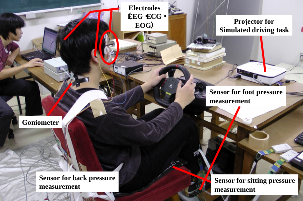
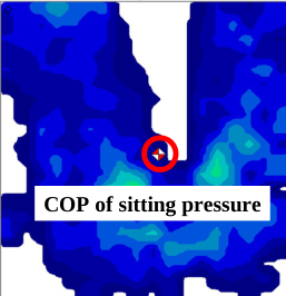
Apparatus Electroencephalography (EEG) led from O1 and O2, Electrocardiography (ECG) led from V5 and Electrooculography (EOG) were acquired with A/D instrument PowerLab8/30 and bio-amplifier ML132. EEG, ECG, and EOG were sampled with a sampling frequency of 1kHz. The photo of experimental settings and the outline of experimental setup (apparatus) are shown in Figure 1 and Figure 2, respectively. The example of COP
Electrodes (EEG・ECG・ EOG)
Projector for Simulated driving task
Sensor for foot pressure measurement
Goniometer
Sensor for back pressure measurement
Sensor for sitting pressure measurement
1
Figure 1. Photo of experimental setting.
PC for sitting pressure measurement (Comfolight)
Neck bending angle
PC Participant PC for back and foot Pressure measurement (Octsense)
PC PC
EOG
Power Lab Bioamp
ECG⇒RRV3 EEG⇒MPF
PC for tracking task
PC PC
PC
Steering Switch
PC for biological measurement
Projector for simulated driving task
Figure 2. Outline of experimental setup.
Figure available in the original PDF paper.
(Center of Pressure) measurement on the sitting surface, the setting for back pressure measurement, and the setting for foot pressure measurement are shown in Figure 3.
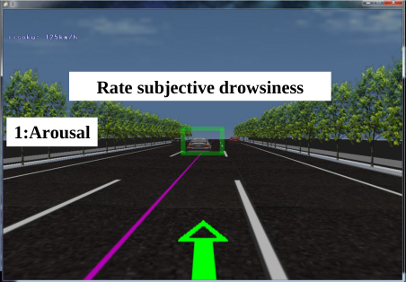
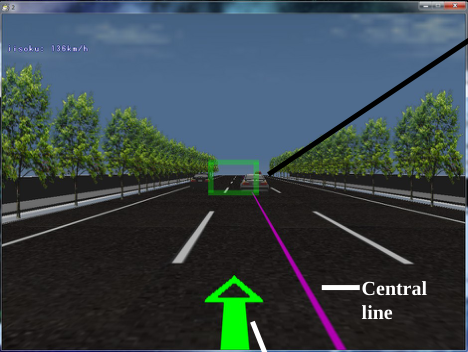
Task The participants sat on an automobile seat, and were required to carry out a simulated driving task. For both conditions (low arousal and high arousal conditions), the participants were required to carry out a simulated driving task. The display of the driving simulator is depicted in Figure 4. The participants were required to steer a steering wheel and keep their vehicle to the center line (purple color) as much as they could. Three types of the distances between two cars are demonstrated in Figure 5. If the participant kept the distance between two cars to a moderate level, the following car was encompassed by a green rectangle. If the distance between two cars was too short or too long, the color of the encompassed rectangle changed to different color (red for short distance or blue for long distance between two cars) as in Figure 5.
COP of sitting pressure COP of sitting pressure
Setting for back pressure measurement
Masurment of COP on sitting surface
Setting for foot pressure measurement
Figure 3. Demonstration of COP measurement on sitting surface, setting for back pressure measurement, and setting for foot pressure measurement.
Sampling intercval of tracking data:1Hz
1
Rate subjective drowsiness
2
1:Arousal
3
1:arousal 2:a little drowsy 3:very drowsy (0:No pressing) Road width From Center of running lane to the edge of the road: 7.5m(3.5+ 1.75+ 2.25)
Figure 4. Display of simulated driving task, and switches for drowsiness evaluation.
The psychological rating included the following three categories: 1: arousal, 2: a little drowsy, 3: very drowsy. The participant was required to evaluate his drowsiness using the switches 1-3 in Figure 4 every one minute.
Procedure and Data Processing Before the EEG data were entered into FFT program, the data were passed through a cosine taper window. FFT was carried out every 1024 data (1.024s). The mean power frequency was calculated. The moving average per ten inter- beta intervals was calculated. Variance of past three inter-beat intervals was calculated as RRV3, which is regarded to represent the functions of parasympathetic nervous systems. The relation between these measurements and
Precedent car Distance between two cars: proper
Distance between two cars: short
Central line
Distance between two cars: long
Controlled object
Figure 5. Three distance conditions( proper, short, and long) in simulated driving task.
Subjective drowsiness Predicted value ◇ Measured value ■ Measured data
Quantity of Pedal operation RRV3 Movement of COP
Neck bending angle (Horizontal) Neck bending angle (Vertical) Back pressure
Frequency of body movement
Figure 6. Concept of prediction of drowsiness. Subjective drowsiness is predicted by applying multinomial logistic regression to measured data.
Figure available in the original PDF paper.
subjective drowsiness was analyzed. The psychological rating of drowsiness checked every 1 min in order to use this as a baseline of change of drowsiness with time. EEG- MPF, RRV3, the number of blinks, and the mean tracking error were obtained every one minute.
As for behavioral measures, neck vending angle (horizontal and vertical), back pressure, foot pressure, COP on sitting surface, frequency of body movement, tracking error in driving simulator task, and standard deviation of quantity of pedal operation were measured (see Figure 1 and Figure 3). The neck bending angle was sampled with the sampling frequency of 1kHz. ECG and EOG were resampled with the sampling frequency of 100Hz. The foot pressure, the back pressure, and COP on sitting surface were sampled with the sampling frequency of 2Hz. The quantity of pedal operation and the tracking error were measured every one second (sampling frequency of 1Hz).
Prediction of drowsiness at present Previous prediction point in time
t
60s
20s
Length of interval used for prediction 0s 10s~100s
Figure 7. Explanation of prediction scheme on the basis of past intervals.
Figure available in the original PDF paper.
Physiological and behavioral measures above were recorded while performing a simulated driving task for (at most) one hour. Applying these measures to the multinomial logistic regression models, the prediction accuracy of drowsiness was compared among a variety of combinations of physiological and behavioral evaluation measures (see Figure 12).
The procedure for predicting subjective drowsiness is summarized in Figure 6. An attempt was made to predict subjective drowsiness by applying multinomial logistic regression to measured data. Measured data included the following physiological measures: x1:RRV3, x2: MPF, and x3: blink frequency. The following behavioral measures were also included in measured data: x4:tracking error in simulated driving task, x5: body movement, x6:neck bending angle (horizontal), x7:neck bending angle (vertical), x8:back pressure, x9: foot pressure, x10:movement of COP, and x11:S.D. (standard deviation) of quantity of pedal operation.
The prediction was carried out according to the scheme in Figure 7. The prediction of the drowsiness rating was conducted using measures before 20-120 s of the prediction. The analysis interval ranged from 10 s to 100 s. The following ten different analysis intervals were used: -30s to -20s (10s-interval), -40s to -20s, -50s to -20s, -60s to - 20s, -70s to -20s, -80s to -20s, -90s to -20s, -100s to -20s, -110s to -20s, and -120s to -20s ( 100s-interval). The interval ranged from 10s to 100s. The effect of the interval used for the prediction on the prediction accuracy was explored. The data 20s before the prediction was used, because we judged that it took at least 20s to take a proper measure for preventing drowsy driving.
RESULTS
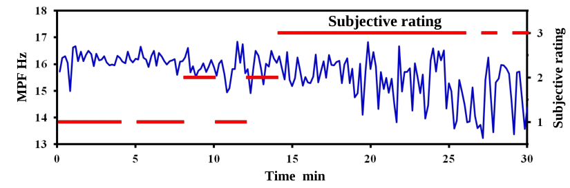
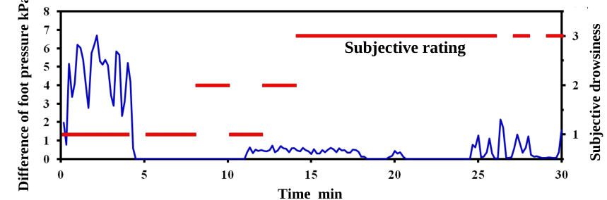
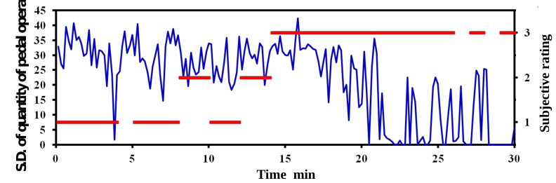
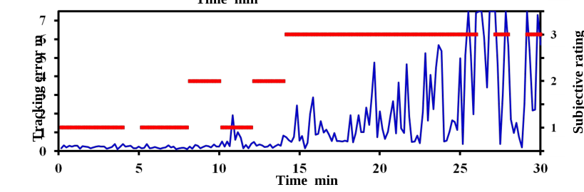
The change of MPF obtained from spectral analysis of EEG time series over time is shown in Figure 8. The upper corresponds to the change when drowsiness is not induced (the participant is arousal, and doesn’t feel drowsy). The lower corresponds to the change when drowsiness is induced. The change of difference of foot pressure over time is plotted in Figure 9. The upper corresponds to the case when drowsiness is not induced. The lower corresponds to the case when drowsiness is induced. The change of S.D. of quantity of pedal operation over time is shown in Figure 10. The upper is the change of this measure when drowsiness is not induced. The lower corresponds to the case when drowsiness is induced. The change of tracking error over time is plotted in Figure 11. The upper is the change of this
Figure 8. Change of MPF obtained from spectral analysis of EEG time series over time. Upper: when drowsiness is not induced. Lower: when drowsiness is induced.
Subjective rating
(Participant D)
Subjective drowsiness Subjective drowsiness
Time min
Subjective rating
Subjective drowsiness Subjective drowsiness
Difference of foot pressure kPa Difference of foot pressure kPa
Time min
Figure 9. Change of difference of foot pressure over time. Upper: when drowsiness is not induced. Lower: when drowsiness is induced.
Subjective rating Subjective rating
Time min
(Participant D)
Subjective rating Subjective rating
S.D. of quantity of pedal operation S.D. of quantity of pedal operation
Time min
Figure 10. Change of S.D. of quantity of pedal operation over time. Upper: when drowsiness is not induced. Lower: when drowsiness is induced.
Figure 12. Prediction accuracy of drowsiness prediction compared among a variety of combinations of evaluation measures. Drowsiness was predicted using a multi-nominal logistic regression model.
Figure available in the original PDF paper.
Prediction accuracy
Participant (11 measures)
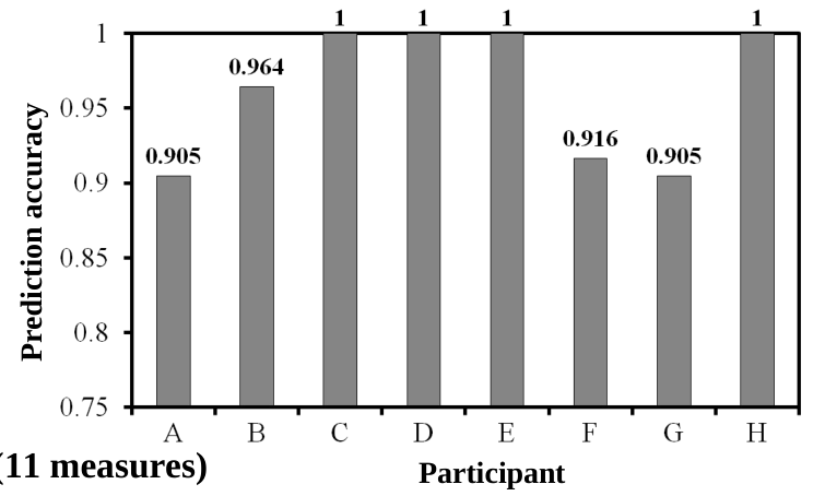
Figure 13. Prediction accuracy compared among eight participants A-H.
Prediction accuracy
Data analysis interval s
(11 measures)
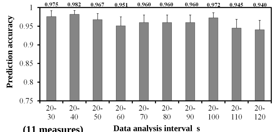
Figure 14. Prediction accuracy of drowsiness prediction compared among a variety of combinations of evaluation measures. Drowsiness was predicted using a multi-nominal logistic regression model.
measure over time under highly arousal state. The tracking error constantly took smaller values. The lower is the change of tracking error over time under highly drowsy state.
In Figure 12, the prediction accuracy of drowsiness every one minute is compared among 13 combinations ((a)-(m)) of physiological and behavioral measures. In Figure 13, the prediction accuracy when 11 measures were used for the prediction is compared among eight participants. Figure 14 compares the prediction accuracy among 10 intervals (from 10s to 100s).
DISCUSSION
The change of MPF obtained from spectral analysis of EEG time series is shown in Figure 8. The upper corresponds to the change when drowsiness is not induced. The lower corresponds to the change when drowsiness is induced. When the drowsiness was not induced, the subjective rating of drowsiness was constantly “arousal.” In accordance with this tendency, MPF was almost constant, and did not change remarkable. On the other hand, the following tendency was observed. Under such a situation, the subjective drowsiness rating 3 (“drowsy”) increased after 15 minutes. The missing value of subjective drowsiness rating means that the participant missed pressing the switch due to excessive drowsiness.
The change of difference of foot pressure is plotted in Figure 9. The upper corresponds to the case when drowsiness is not induced. The lower corresponds to the case when drowsiness is induced. When the drowsiness is not induced, the difference of foot pressure did not change in accordance with the constant subjective rating of drowsiness (“arousal”). When the arousal level decreased and drowsiness was induced to a larger extent, the difference of foot pressure considerably decreased accordingly. The subjective rating on drowsiness belonged to 3 (“very drowsy”) after 14 minute, and the value of difference of foot pressure got smaller and smaller.
The change of S.D. of quantity of pedal operation over time is shown in Figure 10. The upper is the change of this measure when drowsiness is not induced. The lower corresponds to the case when drowsiness is induced. When drowsiness is not induced, S.D. of quantity of pedal operation decreased.
The change of tracking error over time is plotted in Figure 11. The upper is the change of this measure over time under highly arousal state. The tracking error constantly took smaller values. The lower is the change of tracking error over time under highly drowsy state. With the accumulated drowsiness, it trended that the tracking error increased.
From the examples of three evaluation measures, it has been demonstrated these measures sensitively react to the change of arousal level. Therefore, as a next step, an attempt was made to predict subjective rating on drowsiness according to the procedure shown in 7. In this study, as mentioned above, ten kinds of intervals (from 10s (-30s to - 20s)) to 100s (-120s to -20s)) used for predicting drowsiness before 20s.
The following multinomial logistic regression was used to predict the subjective drowsiness expressed from 1 (“arousal”) to 3 (“very drowsy”). The dependent variable was the subjective drowsiness, and the independent variables corresponded to 11 measures above mentioned.
0 1 1 11 11
b b x b x P b b x b x
exp( (2) (2) (2:a little drowsy)= (1) exp( (2) (2)
Equations and mathematical formulas are available in the original paper PDF.
) 1+ )
0 1 1 11 11
0 1 1 11 11
b b x b x P b b x b x
exp( (3) (3) (3: very drowsy)= (2) exp( (3) (3)
Equations and mathematical formulas are available in the original paper PDF.
) 1+ )
0 1 1 11 11
P
(1:ar
ousal) 1 (2:a little drowsy) (3: very drowsy) (3) P P [Equation or mathematical symbol available in the original paper PDF][Equation or mathematical symbol available in the original paper PDF] Here x1:RRV3, x2:MPF, and x3: blink frequency, x4:tracking error in simulated driving task, x5: body movement, x6:neck bending angle (horizontal), x7:neck bending angle (vertical), x8:back pressure, x9: foot pressure, x10:movement of COP, and x11:S.D. (standard deviation) of quantity of pedal operation. x1(2), ……., x11(2) show the value of each evaluation measure when the corresponding subjective evaluation is equal to 2. x1(3), ……., x11(3) show the value of each evaluation measure when the corresponding subjective evaluation is equal to 3. According to the calculated probability P(1), P(2), and P(3), the prediction of the subjective drowsiness was conducted. The prediction accuracy thus obtained is discussed below from the viewpoints of what combination of 11 measures is desirable, how the individual differences are included in the prediction results, and what interval out of 10 intervals ((-30s, -20s), …… (-120s, -20s)) leads to higher prediction accuracy.
In Figure 12, the prediction accuracy of drowsiness every one minute is compared among 13 combinations ((a)-(m)) of physiological and behavioral measures. The graph shows that the mean prediction accuracy was the highest when all of 11 measures were entered into the multinomial logistic regression model ((a) in Figure 12). The prediction accuracy was the lowest when only physiological measures were used ((m) in Figure 12). The prediction accuracies for (a), (b), and (c) in Figure 12 were nearly the same, which means that COP movement on the sitting surface, S.D. of pedal operation, and the frequency of body movement do not contribute to the enhancement of the prediction accuracy. Moreover, this indicates that the combination (c) is desirable, because the high prediction accuracy was obtained with fewer behavioral measures. Although higher prediction accuracy more than 0.9 was as a whole obtained, the combinations (a), (b), and (c) certainly assured higher prediction accuracy more than 0.96. From the practical viewpoint, however, it might be difficult to use 11 measures and install the measurement system for these 11 measures. Therefore, future research should pursuit stingy and economic approach which assures higher accuracy so that such a system can be put into practical use.
In summary, these results mean that using behavioral measures together with physiological measures leads to high prediction accuracy. As a result of exploring the possibility of driver’s drowsiness prediction with high accuracy using both physiological and behavioral measures, we can conclude that such an approach is promising and leads to higher prediction accuracy.
In Figure 13, the prediction accuracy when 11 measures were used for the prediction is compared among eight participants. This shows that there exist larger individual differences in the prediction accuracy. The prediction accuracy was perfect for the participants C, D, E, and H, while the prediction accuracy for the participants A, B, F, and G were about 0.9 and not so high like those for C, D, E, and H. The reason can be discussed as follows. Analyzing the experimental situation (change of evaluation measures, video images during the experiment, and the missing of switch pressing) of each participant, the degree of drowsiness for the participants C, D, E, and H was more remarkable than that for the participants A, B, F, and G.
Figure 14 compares the prediction accuracy among 10 intervals (from 10s to 100s). As a whole, the interval from -40s to -20s led to the highest prediction accuracy (0.982). As shown in Figure 14, the interval which is far from the point in time for prediction did not lead to high prediction accuracy as compared with the interval near to the point in time for prediction (intervals -30s to -20s, -40s to -20s, and -50s to -20s). The results show that the selection of interval used for drowsiness prediction affected the prediction accuracy. The most proper interval must be from -40 to -20s. Future research should develop faster processing (prediction) technique when putting the prediction method into practice.
Although the prediction of subjective drowsiness was carried out in this study and it has been shown that the proposed method can reliably and accurately predict the timing when the participant feel subjectively drowsy, it is further necessary to identify the time when the driver is sure to fall into asleep and at worst case bring about a crucial traffic accident, and explore whether it is possible to predict such timing in advance using the measures adopted in this study. Such identification of the timing when the driver is sure to fall into asleep and at worst case bring about a crucial traffic accident is essential for the prevention of crucial traffic accidents due to drowsy driving. The result in this study would be effective as a base of such an approach.
CONCLUSIONS
As a result of predicting subjective drowsiness using multinomial logistic regression where dependent variable and independent variables were subjective drowsiness rating (1, 2, and 3) and measures x1 to x11, respectively, a high prediction accuracy more that 0.9 was attained. Moreover, the interval from -40s to -20s before prediction point in time was found to enhance prediction accuracy more than 0.98.
From the practical point of view, it is desirable that the higher prediction accuracy should be achieved with only behavioral measures, because the physiological measures are not cost-efficient and might be difficult to use practically. Future research should explore the practical use of drowsiness prediction system using only behavioral measures.
REFERENCES
Brookhuis, K. A. and Waard,D. (1993), “The use of psychophysiology to assess driver status”, Ergonomics, Vol.36, pp.1099-
1110. Kecklund, G. and Akersted, T. (1993), “Sleepiness in long distance truck driving: An ambulatory EEG study of night driving”, Ergonomics, Vol.36, pp.1007-1017. Murata, A. and Hiramatsu, Y. (2008), “Evaluation of drowsiness by HRV measures -Basic study for drowsy driver detection-“,
Proc. of IWCIA2008, pp.99-102. Murata, A., Koriyama, T. and Hayami, T. (2012), “Basic Study on the Prevention of Drowsy Driving using the Change of Neck Bending Angle and the Sitting Pressure Distribution”, Proc. of SICE2012, pp.274-279. Murata, A., Koriyama, T., Ohkubo, Y., Moriwaka, M. and Hayamai, T. (2013a), “Verification of Physiological or Behavioral
Evaluation Measures Suitable for Predicting Drivers’ Drowsiness”, Proceedings of SICE2013, pp.1766-1771. Murata, A., Matsuda, Y., Moriwaka, M. and Hayami, T. (2011), “An Attempt to predict drowsiness by Bayesian estimation”, Proc. of SICE2011, pp.58-63. Murata, A., Nakatsuka, A. and Moriwaka, M. (2013b), “Effectiveness of Back and Foot Pressures for Assessing Drowsiness of
Drivers”, Proceedings of SICE2013, pp.1754-1759. Murata, A. and Nishijima, K. (2008), “Evaluation of Drowsiness by EEG analysis -Basic Study on ITS Development for the Prevention of Drowsy Driving-“, Proc. of IWCIA2008, pp.95-98. Murata, A., Ohkubo, Y., Moriwaka, M. and Hayami, T. (2011), “Prediction of drowsiness using multivariate analysis of
biological information and driving performance”, Proc. of SICE2011, pp.52-57. Murata, A., Urakami, Y., Koriyama, T., Ikeda, M. and Hayami, T. (2013c), “Evaluation of Drowsiness of Driver Based on Change of Sitting Pressure Center”, Proceedings of SICE2013, pp.1760-1765. Skipper, J. H. and Wierwillie, W. (1986), “Drowsy driver detection using discrimination analysis”, Human Factors, Vol.28,
pp.527-540.
LISTED IN THE AHFE DIGITAL BOOKSTORE CATALOGUE
Explore the complete digital volume
Advances in Safety Management and Human Factors
Read this individual research paper free through the original publisher, or explore the full digital proceedings book.
ISBN 978-1-4951-2100-5
Explore this ISBN in the AHFE Bookstore ↗Listed in the July 2026 bookstore catalogue; search by ISBN to confirm current availability · Digital book purchase optional