Ian Tassin, Patrick J. Donnelly (2026). Toward Better Machine Understanding of Rhythm: Rhythmicness as a Regression Problem. In: Human Interaction and Emerging Technologies (IHIET-AI 2026): Artificial Intelligence and Future Applications. AHFE Open Access, vol. 201, pp. 653–664. https://doi.org/10.54941/ahfe1007220
The concept of musicality refers to the ambiguously defined qualities of melodiousness, harmoniousness, and rhythmicity. Prior computational research has investigated musicality solely as a classification task discriminating music from speech or other environmental sounds, however, research in psychoacoustics indicates that people perceive musicality as a continuous rather than discrete feature audio. To address this, we propose a novel task of assessing musicality, and the absence thereof, as a continuous feature of sound. We present novel datasets and a regressive approach for assessing the extent to which a given piece of audio contains a structured rhythm. We test a variety of convolutional models, including a state-of-the-art model from the related task of beat-tracking, to try and predict the extent to which a given audio sample differs from a metrically regular pattern of note onsets. We make contributions toward determining which models are suited for this task, and establish model performance baselines for future research on this task.
Prior work has focused on classifying either music (Oramas et al., 2018; Nieto et al. 2020) or environmental sounds (Piczak, 2015; Mu et al. 2021), or on broadly discriminating musical from non-musical sounds (Alías et al. 2016; Bhattacharjee et al. 2018; Gemmeke et al. 2017), rather than treating musicality as an inherent feature which all sound possesses to varying extent. We argue that we should instead determine the extent to which an individual sound is musical or not-musical. This view better aligns with a large body of research from musicology and psychoacoustics that indicates people do not only perceive "music" and "not music", but rather they interpret a variety of different features that contribute to the perception of sounds as more or less musical (Margulis et al. 2016, Møller et al. 2021; Simchy-Gross et al. 2018; Vuust et al 2022). In machine learning research, musical features are generally considered for music- specific tasks like music genre (Pelchat et al. 2020) or emotion classification (Han et al. 2022), but there is no active body of research that considers musical features to exist in non-musical sounds. This deficiency persists despite the fact that research shows that examples of traditionally non-music sounds can be perceived as musical (Deutsch et al. 2011; Simchy-Gross et al. 2018; Rhimmon et al. 2018).
A related challenge is that existing audio features require manual annotation and are subject to cultural and individual biases (Fu et al. 2011; Aljanaki et al. 2014; Flexer et al. 2021; Yang et al. 2023; Watcharasupat et al. 2025; Panda et al. 2023), limiting the availability of high-quality large-scale datasets. In this work we introduce data generation techniques that have the potential to support automated feature extraction for novel features which are important to human music perception.
Furthermore, we are influenced by the literature exploring time-series forecasting (Dong et al. 2025) and the task of beat-tracking (Davies et al. 2009; Jia et al. 2019; Zhao et al. 2022). Time-series forecasting is the class of problems concerned with predicting future events based on past data. Research indicates that humans' ability to accurately perform time-series forecasting with sound events is integral to the experience of sound as musical (Vuust et al. 2022). Motivated by this fact, we design experiments with a model architecture designed for time-series forecasting tasks: the Fourier Analysis Network (FAN) (Dong et al. 2025). Dong et al. originally proposed this architecture and demonstrate that it can offer improved performance compared to other methods, such as simple MLP and transformers, for time-series forecasting problems.
Beat tracking algorithms and computational models attempt to automatically identify the positions of metric beats in music (Foscarin et al. 2024). Often, beat- tracking models also perform time-series forecasting to predict future beats based on past ones. These approaches are concerned with the identification of note onsets in order to map them to the most likely rhythmic beats. We borrow from this area of research and adapt to our task the architecture of one such state-of- the-art model designed for beat tracking, the BeatTransformer by Zhao et al. (Zhao et al. 2022). Additionally, when choosing the representations of our data and our model architecture for our experimental learning, we rely on existing
655 Tassin and Donnelly
research that indicates that mel-spectrograms are a suitable audio representation, rather than relying on the higher-dimensionality of raw audio signals (Dai et al. 2017; Stowell 2022). In this work, we introduce the novel task of determining the extent to which a given piece of audio has an expected rhythmic structure, generating novel datasets that perturb musicality along four key dimensions: pitch, duration, loudness, and note onset timing. We then compare an array of deep learning architectures to predict the amount of onset perturbation, which we show relates to the structuredness of the rhythm, and present results indicating what kind of model architecture and dataset formation decisions lead to better results.
DATASETS To support our experiments, we create two datasets of short musical excerpts: one played on piano and one synthesized with randomly chosen MIDI instruments. For both datasets we perturb the musicality of samples along four dimensions: pitch, duration, dynamic level, and note onset. We generate short MIDI sequences of musically plausible song excerpts, each featuring a pattern of random notes within a specific musical key, uniquely generated per example by random seeds controlling the number of notes, key, pitches, interval pattern, pitch range, note duration, dynamic level (MIDI velocity), and tempo (BPM). This pattern is repeated to exceed our target duration of six seconds. Crucially, each un-perturbed sample has a constant interval between notes, giving it a perfectly regular rhythmic structure.
We then perturb each example by modifying individual note pitches, durations, loudness, and onset timing, with the amount of perturbation along each dimension controlled by randomized seeds. Alongside each generated MIDI file, we save these values to document the amount of perturbation applied.
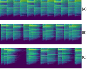
Onset Perturbation For the purposes of this initial investigation, we seek to predict the amount of onset perturbation and we treat the perturbations in other dimensions as noise added to the dataset. Specifically, our empirical task is to determine how much onset perturbation has been applied to an audio sample, given only the perturbed audio as input. To illustrate the effects of note perturbation, we produce an audio example with different levels of perturbation, as shown in Figure 1.
More formally, onset perturbation is defined as follows. Given a sequence of sounds such that where each denotes the time that the sound in begins. Assume has a perfectly regular rhythmic structure, meaning . That is to say, all sound onsets occur with exactly time between them and this assumption holds for the MIDI files we generate prior to applying perturbations. Now assume we have some
such that each where is a random value sampled from a uniform distribution in range , where is a parameter set before sequence is generated. Onset perturbation is calculated by Equation 1, which leads us to Equation 2. In practice, we do not allow noise to be applied
Toward Better Machine Understanding of Rhythm 656
such that . Since this has no major impact on the resulting audio, we omit this detail from the calculations for simplicity. The constant in the calculation simply converts the value to a percentage.
Importantly, because we arrive at Equation 3. This means, in the expectation, we avoid edge cases where a large majority of sound events are moved forward or backward in time. Additionally, since any two note perturbations and are expected to have different values , as seen by , we are safe to assume that, in the expectation for , and therefore, the perturbed sound sequence no longer has a perfectly regular rhythmic structure.
Figure 1: Illustration of the same example with 0%, 25.73%, and 50.31% onset perturbation, with no other perturbations applied. Notes are rendered on the piano and represent the sequence C♯4- G♯3-A♯3-F♯3 repeated three times. Note: this example shows a single audio clip at multiple levels of perturbation for the sake of illustration, but the dataset we use does not contain duplicate audio at multiple perturbation levels, and does not store the original unperturbed audio.
Equation 1: onset perturbation
Equation 2: expected onset perturbation
Equation 3: expected Dataset Splits After applying perturbations, we synthesize each MIDI example as a .wav file, truncate each excerpt to six seconds, and convert the audio to mel-spectrograms. We transform each spectrogram from RGB to LAB color-space, which has been shown to increase model performance in certain image tasks (Gowda et al. 2018), and save them as .npy files with dimensions , in which the multiplier refers to the color dimensions.
657 Tassin and Donnelly
The piano dataset contains 10,000 examples split into training (n=9000) and test (n=1000) sets. The instrument dataset is similar except that 24 examples were discarded because some instruments produced silent notes under certain conditions, resulting in training (n=8978) and test (n=998) sets.
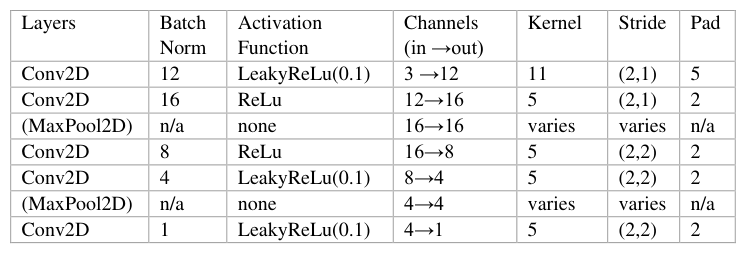
MODEL ARCHITECTURES For our empirical evaluations we test a large array of model architecture variations. The majority of these models use CNN-based architecture. We expand upon a baseline CNN, exploring different types of pooling layers and other modifications to create a large set of convolutional models for use in our experiments. In addition to the CNN variants, we modify the BeatTransformer model based on the architecture presented in (Zhao et al. 2022). This is the only model we investigate that does not build off of the baseline CNN architecture we present in Table 1.
Table 1. General model architecture of the CNN models. The optional MaxPool2D layers shown in parentheses are only included in the pooling methods variants.
CNN+Linear Our first variant builds upon the baseline CNN architecture by adding a series of fully-connected layers. Following the convolutional layers specified in Table 1, the output is first flattened to size then connected to three fully connected layers with dimensions: , , , and . We include LeakyReLU activation functions between each linear layer with negative slope set to .
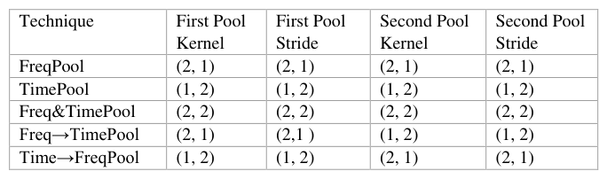
Pooling Methods Next, we modify the CNN+Linear model to explore the effects of different pooling techniques. Specifically, we wish to investigate potential differences by pooling in the frequency dimensions (height) versus pooling in the time dimension (width). We consider the placement of two pooling layers: one early, following the convolutional layer, and another later, following the convolutional layer (see Table 1). We consider different combinations for pooling in the frequency and time dimensions and we list the five different pooling strategies in Table 2. These include pooling in the frequency dimension (FreqPool), pooling in the time dimension (TimePool), pooling in both frequency and time (Freq&TimePool), pooling frequency early and then later pooling in
Toward Better Machine Understanding of Rhythm 658
time (Freq→TimePool), and early pooling in time followed by late pooling in frequency (Time→FreqPool).
Table 2. Summary of the different pooling approaches illustrating the kernel size and stride for each of the two pooling layers.
CNN+FAN A Fourier Analysis Network (FAN) layer is a modified form of a neural network layer proposed by Dong et al. (Dong et al. 2025) that integrates the Fourier principle into the network structure. The authors found that FAN layers can be useful for time-series forecasting and other tasks which exhibit some periodic structure in the data. We investigate the inclusion of this layer because we are concerned with how our onset perturbation disrupts the expected periodicity of the musical sequence.
To incorporate the FAN layer, we flatten the output from the baseline CNN model (see Table 1) to a vector of size 1024. This is then connected to two FAN layers, of dimensions and , followed by two linear layers of dimensions and . A LeakyReLU with negative slope is used after the second linear layer. No activation functions are added between FAN layers, since the FAN architecture itself uses pre-specified activation functions.
BeatTransformer Lastly, we compare our various CNN models to the BeatTransformer model, a state-of-the-art model used for beat detection and downbeat tracking (Zhao et al. 2022). Notably, we make several small modifications to the original architecture in order to create a modified BeatTransformer that can operate on our task. In particular, our task necessitates different input and output dimensions, and we made adjustments accordingly. Our input size is and the output of our regression problem is a float value. Additionally, we also modify the ReLU activation functions of the original architecture from (Zhao et al. 2022) to be LeakyReLU activation functions with negative slope 0.1 in the CNN layers to improve gradient propagation. The original architecture (Zhao et al. 2022) contains two output vectors and . Because we are only interested in a single float value output for our regression task, we concatenate them into a single vector then run through linear layers with dimensions , , and to obtain output predictions.
659 Tassin and Donnelly
RESULTS AND DISCUSSION We conduct experiments across both datasets using L1 loss and a learning rate of 0.0008 for all models. For the BeatTransformer model, we applied gradient clipping with max_norm=1.0 to ensure training stability. All models are trained for 50 epochs and evaluated on the test set.
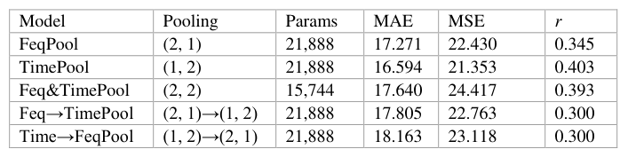
We first compare the primary model architectures: CNN+Linear, CNN+FAN, and BeatTransformer. All models use the base CNN architecture in Table 1 without pooling layers, except for BeatTransformer which uses the architecture from (Zhao et al. 2022). Results are shown in Tables 3 and 4. We then compare the five pooling strategies from Table 2 applied to our CNN+Linear architecture, pooling in either the frequency dimension (spectrogram height), time dimension (spectrogram width), or both, with results in Tables 5 and 6.
Architecture Experiment Results For both datasets, we observe comparable performance between the CNN+Linear (Pearson's r=0.570) and CNN+FAN (r=0.571) models. On the piano only task, the performance of the CNN models are relatively comparable to that of the BeatTransformer (r=0.602) model (see Table 3). However, for the instrument variation task, the CNN models (r=0.282 and 0.284) significantly underperform compared to the BeatTransformer (r=0.546) model (see Table 4).
In general, we observe reduced performance across all the models on the instrument dataset compared to the piano dataset. This confirms that the increased variety of different timbres in the instrument dataset is a much more difficult task compared to the single timbre present in the piano only dataset.
Table 3. Comparison of models on the piano-only dataset for the regression task.Table 4. Comparison of models on the instrument dataset for the regression task.
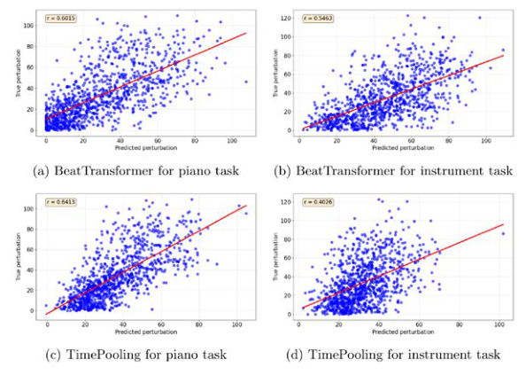
Pooling Experiment Results For the piano-only task, TimePool, Feq&TimePool, and Feq→TimePool slightly outperform the other strategies (Table 5), however Feq→TimePool suffers more than the others on the instrument task. As with the primary architecture comparison, we observe a significant performance drop across all models on the instrument task (Table 6), with TimePool performing best overall (r=0.403), despite a significant reduction from its piano-only performance (r=0.641). Notably, all pooling models outperform the non-pooling CNN models across
Toward Better Machine Understanding of Rhythm 660
both datasets, and since TimePool performs best on the harder instrument task, we consider it the best CNN model overall, eclipsed only by BeatTransformer. Scatter plots of predicted versus true perturbation values for these two models are shown in Figure 2.
Table 5 Comparison of models on the piano dataset for the regression task.
Table 6. Comparison of models on the instrument dataset for the regression task.Figure 2: Scatter plots illustrating model predictions against the true values for the CNN with time- pooling and the BeatTransformer models.
Cross Dataset Evaluation Experiment Results In our final experiments, we evaluate the best performing models (TimePool and BeatTransformer) trained on each dataset (Tables 7 and 8), evaluated on both datasets. Models trained on the instrument task and evaluated on the piano task
661 Tassin and Donnelly
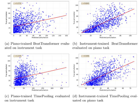
(Table 8) not only outperform those trained on the piano task and evaluated on the instrument task (Table 7), but also outperform models trained and evaluated entirely on the piano task (Table 3). This indicates that training on multiple instruments yields better generalization compared with models trained exclusively on piano.
Figure 3 illustrates this asymmetry: models trained on piano data suffer when evaluated on the instrument dataset (Figure 3, left), while models trained on the instrument dataset generalize well to the piano data (Figure 3, right). The BeatTransformer model trained on the instrument set even outperforms the piano- trained BeatTransformer on the piano-only evaluation data, as can be seen by comparing Figures 3 and 4.
Table 7. Comparison of models trained on the piano dataset and evaluated on the instrument dataset.Table 8. Comparison of models trained on the instrument dataset and evaluated on the piano dataset.Figure 3: Scatter plots depicting model predictions against true values for dataset cross-evaluation experiment.
Toward Better Machine Understanding of Rhythm 662
LIMITATIONS AND FUTURE WORK Despite promising results, we acknowledge several limitations we will address in future work. Our datasets consider four dimensions affecting musicality perception: pitch, duration, dynamic level, and note onset. However, this initial investigation only evaluates onset perturbation. In future work, we will isolate each remaining dimension, supported by a contemporaneous human subject study in which participants determine how each perturbation type affects perceived musicality. Additionally, we currently only investigate monophonic musical lines and intend to extend this approach to polyphonic music to investigate the effects of chord quality and harmony.
Although the instrument dataset experiments were less successful than the piano-only experiments, we believe models trained on instrument variation datasets may better generalize to real-world audio, and we wish to extend this approach to real-world music and environmental sounds. In the long term, we see the potential for models trained on datasets like ours to automatically extract audio features that quantify the structuredness of audio signals, linked to the human ability to predict future sound events within a sample (Vuust et al. 2022).
CONCLUSION We present a new paradigm to explore the machine understanding of sound that more closely aligns with human perceptions of the concept of musicality. We generated novel datasets of piano and mixed instrument sounds in which we systematically alter the musicality of the musical excerpt along the dimensions of pitch, duration, dynamic level, and note onset. In our experiments, we attempt to predict the specific amounts of note onset perturbation for audio samples.
We consider multiple variations of CNN models and found that the inclusion of time pooling layers provides the most improvement compared to other pooling strategies. We also compare these CNN models to the BeatTransformer model (Zhao et al. 2022), a state-of-the-art model for the related problem of beat tracking. We find that it generally outperforms the other models we tested for our task. Across models, we achieved higher results on the single timbre piano-only dataset compared to the instrument dataset, indicating the increased complexity of this problem when considering a large variety of instrument timbres, such as we would find when considering real world music.
Through this work, we develop novel datasets, methods, and evaluation approaches to establish baselines for future research exploring this task of quantifying musicality measured as a continuous spectrum. We hope that this research encourages further empirical investigations into the ability of deep learning models to quantify the subjective question of what makes a sound musical.
REFERENCES Aljanaki, A., Yang, Y.-H., & Soleymani, M. (2014). Emotion in music task at MediaEval
2014. In MediaEval 2014. Alías, F., Socoró, J. C., & Sevillano, X. (2016). A review of physical and perceptual feature extraction techniques for speech, music and environmental sounds. Applied
663 Tassin and Donnelly
Sciences, 6(5). https://doi.org/10.3390/app6050143 Bhattacharjee, M., Prasanna, S. R. M., & Guha, P. (2018). Time-frequency audio features for speech-music classification. arXiv. https://doi.org/10.48550/arXiv.1811.01222 Dai, W., Dai, C., Qu, S., Li, J., & Das, S. (2017). Very deep convolutional neural
networks for raw waveforms. In 2017 IEEE International Conference on Acoustics, Speech and Signal Processing (ICASSP) (pp. 421–425). IEEE. https://doi.org/10.1109/ICASSP.2017.7952190 Davies, M. E. P., Degara, N., & Plumbley, M. D. (2009). Evaluation methods for musical audio beat tracking algorithms (Tech. Rep. No. C4DM-TR-09-06). Queen Mary University of London, Centre for Digital Music. Deutsch, D., Henthorn, T., & Lapidis, R. (2011). Illusory transformation from speech to
song. The Journal of the Acoustical Society of America, 129(4), 2245–2252. https://doi.org/10.1121/1.3562174 Dong, Y., Li, G., Tao, Y., Jiang, X., Zhang, K., Li, J., Deng, J., Su, J., Zhang, J., & Xu, J.
(2025). FAN: Fourier analysis networks. arXiv. https://doi.org/10.48550/arXiv.2410.02675 Flexer, A., Lallai, T., & Rašl, K. (2021). On evaluation of inter- and intra-rater agreement in music recommendation. Transactions of the International Society for Music Information Retrieval, 4(1), 1–12. https://doi.org/10.5334/tismir.107 Foscarin, F., Schlüter, J., & Widmer, G. (2024). Beat this! Accurate beat tracking without
DBN postprocessing. Transactions of the International Society for Music Information Retrieval. https://doi.org/10.48550/arXiv.2407.21658 Fu, Z., Lu, G., Ting, K. M., & Zhang, D. (2011). A survey of audio-based music classification and annotation. IEEE Transactions on Multimedia, 13(2), 303–319. https://doi.org/10.1109/TMM.2010.2098858 Gemmeke, J. F., Ellis, D. P. W., Freedman, D., Jansen, A., Lawrence, W., Moore, R. C.,
Plakal, M., & Ritter, M. (2017). Audio Set: An ontology and human-labeled dataset for audio events. In 2017 IEEE International Conference on Acoustics, Speech and Signal Processing (ICASSP) (pp. 776–780). IEEE. https://doi.org/10.1109/ICASSP.2017.7952261 Gowda, S. N., & Yuan, C. (2018). ColorNet: Investigating the importance of color spaces for image classification. In Proceedings of the Asian Conference on Computer Vision (ACCV 2018) (pp. 581–596). Springer. https://doi.org/10.1007/978-3-030-20870-7_36 Han, D., Kong, Y., Han, J., & Wang, G. (2022). A survey of music emotion recognition.
Frontiers of Computer Science, 16(6), Article 166335. https://doi.org/10.1007/s11704-021-0569-4 Jia, B., Lv, J., & Liu, D. (2019). Deep learning-based automatic downbeat tracking: A brief review. Multimedia Systems, 25(6), 617–638. https://doi.org/10.1007/s00530- 019-00607-x Margulis, E. H., & Simchy-Gross, R. (2016). Repetition enhances the musicality of
randomly generated tone sequences. Music Perception: An Interdisciplinary Journal, 33(4), 509–514. https://doi.org/10.1525/mp.2016.33.4.509 Møller, C., Stupacher, J., Celma-Miralles, A., & Vuust, P. (2021). Beat perception in polyrhythms: Time is structured in binary units. PLOS ONE, 16(8), Article e0252174. https://doi.org/10.1371/journal.pone.0252174 Mu, W., Yin, B., Huang, X., Xu, J., & Du, Z. (2021). Environmental sound classification
using temporal-frequency attention based convolutional neural network. Scientific Reports, 11(1), Article 21552. https://doi.org/10.1038/s41598-021-01045-4 Nieto, O., Mysore, G. J., Wang, C.-I., Smith, J. B. L., Schlüter, J., Grill, T., & McFee, B.
(2020). Audio-based music structure analysis: Current trends, open challenges, and applications. Transactions of the International Society for Music Information Retrieval, 3(1). https://doi.org/10.5334/tismir.54 Oramas, S., Barbieri, F., Nieto Caballero, O., & Serra, X. (2018). Multimodal deep learning for music genre classification. Transactions of the International Society for
Toward Better Machine Understanding of Rhythm 664
Music Information Retrieval, 1(1), 4–21. https://doi.org/10.5334/tismir.10 Panda, R., Malheiro, R., & Paiva, R. P. (2023). Audio features for music emotion recognition: A survey. IEEE Transactions on Affective Computing, 14(1), 68–88. https://doi.org/10.1109/TAFFC.2020.3032373 Pelchat, N., & Gelowitz, C. M. (2020). Neural network music genre classification.
Canadian Journal of Electrical and Computer Engineering, 43(3), 170–173. https://doi.org/10.1109/CJECE.2020.2970144 Piczak, K. J. (2015). ESC: Dataset for environmental sound classification. In Proceedings of the 23rd ACM International Conference on Multimedia (MM '15) (pp. 1015–1018). Association for Computing Machinery. https://doi.org/10.1145/2733373.2806390 Simchy-Gross, R., & Margulis, E. H. (2018). The sound-to-music illusion: Repetition can
musicalize nonspeech sounds. Music & Science, 1, Article 2059204317731992. https://doi.org/10.1177/2059204317731992 Stowell, D. (2022). Computational bioacoustics with deep learning: A review and roadmap. PeerJ, 10, Article e13152. https://doi.org/10.7717/peerj.13152 Vuust, P., Heggli, O. A., Friston, K. J., & Kringelbach, M. L. (2022). Music in the brain.
Nature Reviews Neuroscience, 23(5), 287–305. https://doi.org/10.1038/s41583-022- 00578-5 Watcharasupat, K. N., Ding, Y., Ma, T. A., Seshadri, P., & Lerch, A. (2025). Uncertainty estimation in the real world: A study on music emotion recognition. In Proceedings of the European Conference on Information Retrieval (ECIR 2025) (pp. 218–232). Springer. https://doi.org/10.1007/978-3-031-88711-6_14 Yang, S., Reed, C. N., Chew, E., & Barthet, M. (2023). Examining emotion perception
agreement in live music performance. IEEE Transactions on Affective Computing, 14(2), 1442–1460. https://doi.org/10.1109/TAFFC.2021.3093787 Zhao, J., Xia, G., & Wang, Y. (2022). Beat transformer: Demixed beat and downbeat tracking with dilated self-attention. ar
LISTED IN THE AHFE DIGITAL BOOKSTORE CATALOGUE
Explore the complete digital volume
Human Interaction and Emerging Technologies (IHIET-AI 2026): Artificial Intelligence and Future Applications
Read this individual research paper free through the original publisher, or explore the full digital proceedings book.
ISBN 978-1-964867-77-9
Explore this ISBN in the AHFE Bookstore ↗Listed in the July 2026 bookstore catalogue; search by ISBN to confirm current availability · Digital book purchase optional